无味卡尔曼滤波器(UKF)
1. 介绍
扩展卡尔曼滤波器可以用来解决和高级驾驶、辅助系统和无人驾驶车相关的问题。如果检查带有自动车距保持功能的汽车和巡航控制系统的代码,你会发现里面有扩展卡尔曼滤波器。还有一种方法在这个领域越来越受关注,它叫做无味卡尔曼滤波器,简称 UKF,它的结果更好。UKF 是处理非线性过程模型或非线性测量模型的替代方法,但是 UKF 不会对非线性函数进行线性化处理,它使用所谓的 sigma点来近似概率分布。这有两个优势,sigma点近似非线性转换的效果大部分情况下比线性化更好,它还可以省去计算雅可比矩阵的过程。
2. CTRV运动模型
2.1 运动模型与卡尔曼滤波器
在扩展卡尔曼滤波中,我们使用了恒定速度模型(CV)。恒定速度模型是用于目标跟踪的最基本的运动模型之一。
但还有许多其他模式,包括:
-
恒定转向率和速度幅度模型(CTRV)
-
恒定转向率和加速度(CTRA)
-
恒定转向角和速度(CSAV)
-
恒定曲率和加速度(CCA)
每个模型对对象的运动做出不同的假设。以下内容将基于使用CTRV模型来说明。
可以将这些运动模型中的任何一个与扩展卡尔曼滤波器或无迹卡尔曼滤波器一起使用。
恒速(CV)模型的局限性
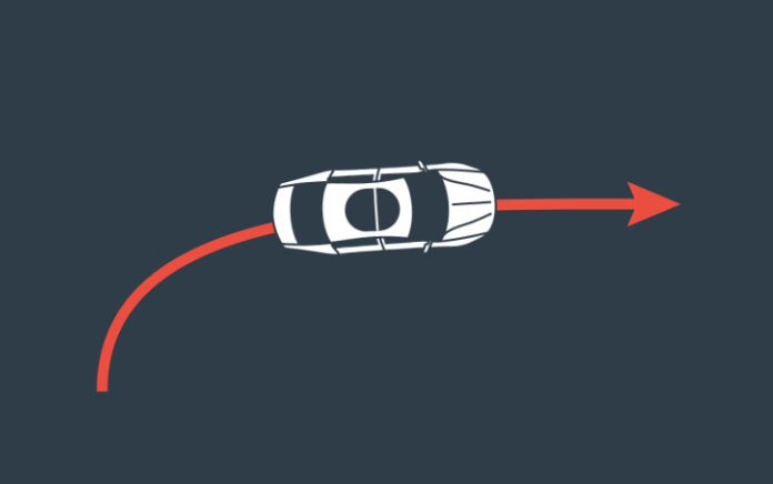
如果假设速度为常量,我们实际上简化了车辆实际移动的方式,因为大多数道路是有拐弯的。因为假设速度为常量的过程模型会因此无法正确预测拐弯车辆。
2.2 CTRV模型状态向量
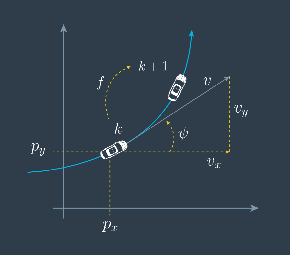
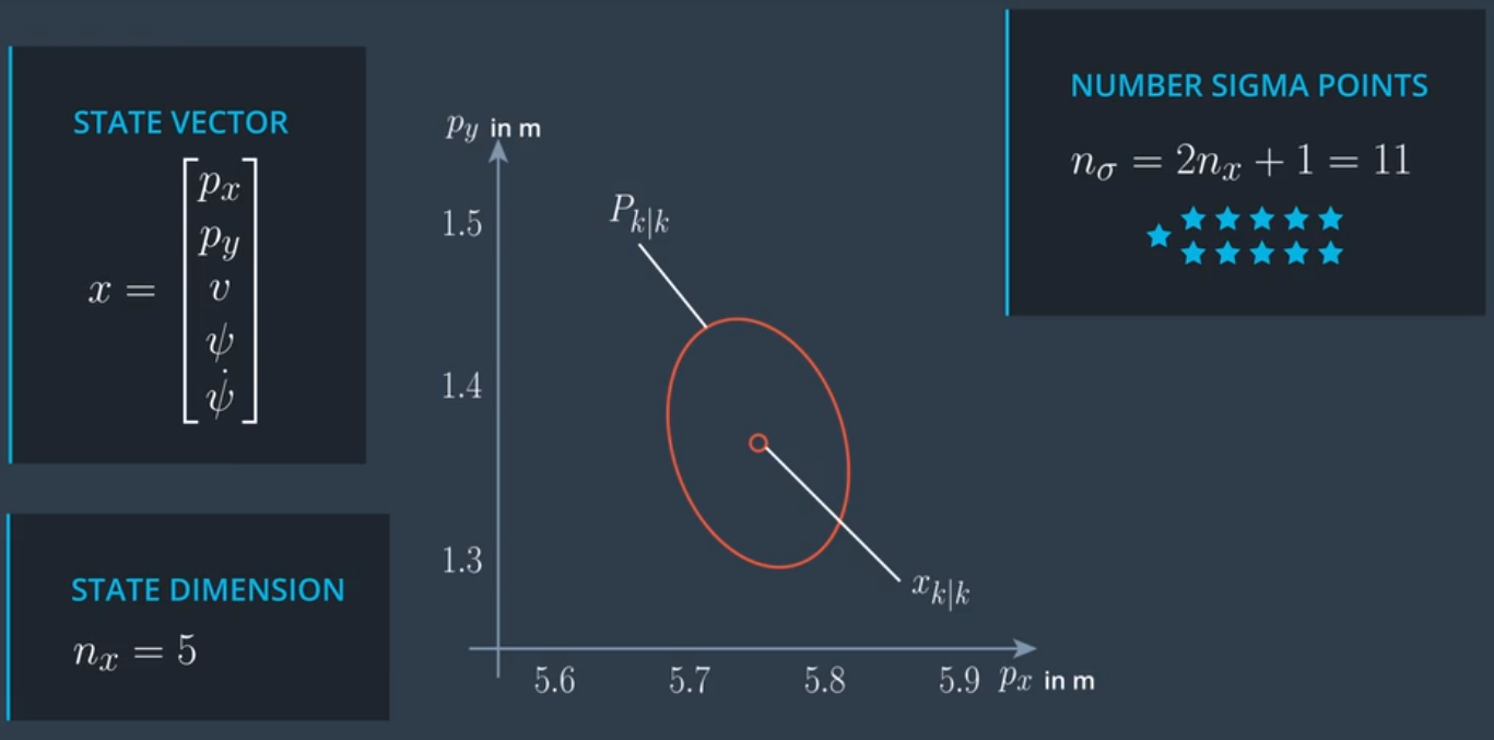
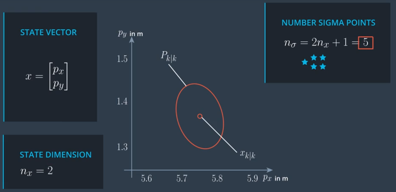
CV模型假设对象沿直线前进, CTRV 模型设对象沿直线前进,同时还能以固定的转弯速率和恒定的速度大小移动。CTRV模型的状态向量用 $p_x$ 和 $p_y$代表二维位置。但是,不用 $v_x$ 和 $v_y$ 表示速度,而是使用速度 $v$ 和偏航角 $ψ$表示,同时能够估算角速度$\dot{\psi}$。恒定的角速度和恒定速度是个好模型,适合真实的交通场景。
\[x = \begin{bmatrix} p_x\\ p_y\\ v\\ \psi\\ \dot{\psi} \end{bmatrix}\]CTRV微分方程
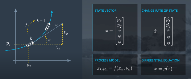
CTRV积分运算
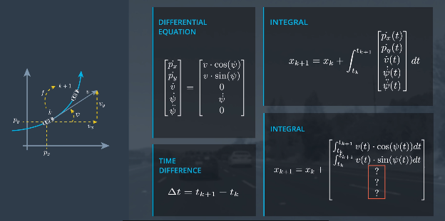
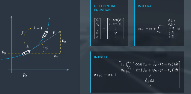
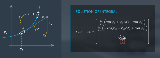
如果$\dot{\psi_k}$是0,也就是当汽车是直线运动时,运动模型的后三个向量都是0,前两个状态向量遵循以下变化。
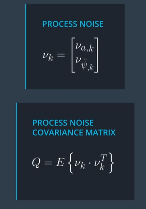
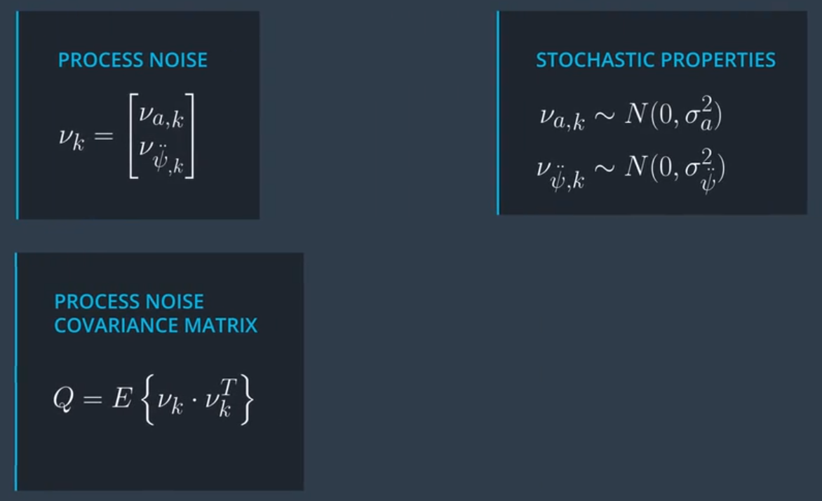
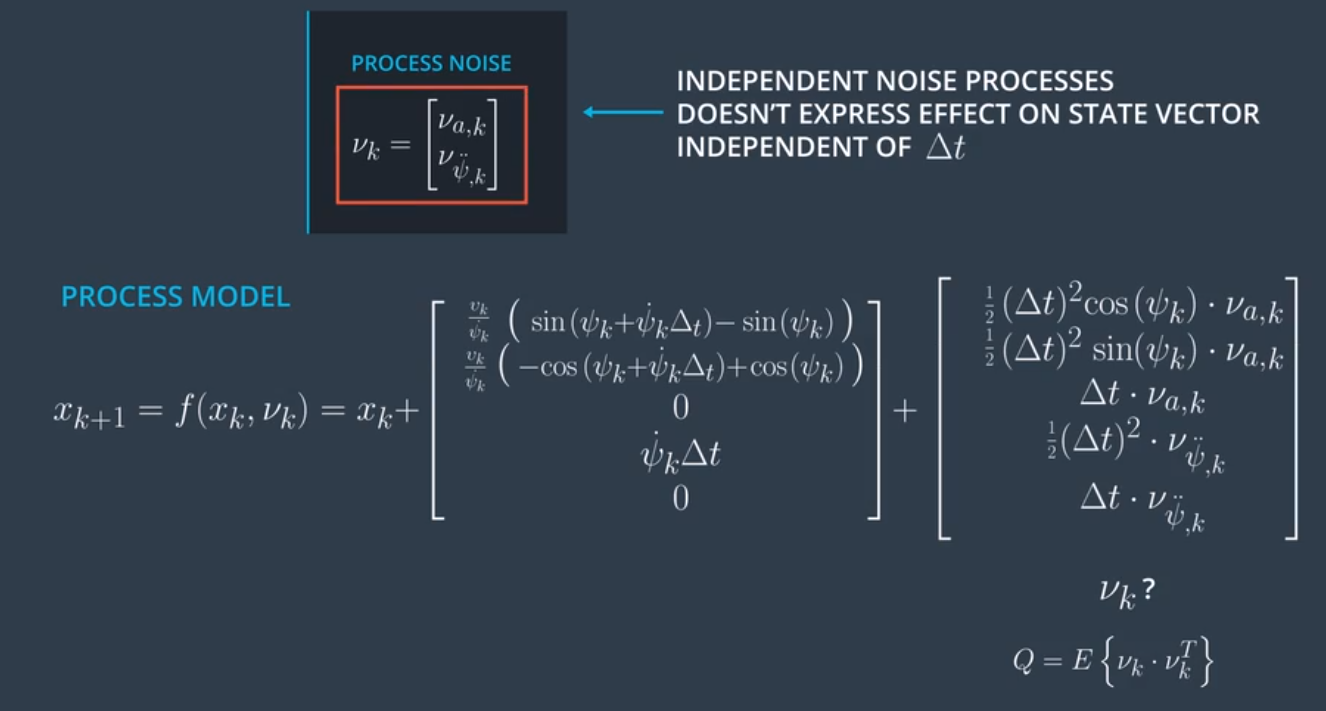
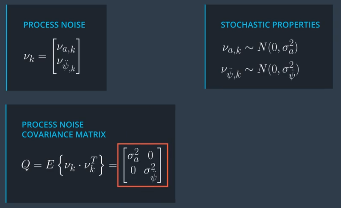
\[v_k cos(\psi_k) \Delta t\] \[v_k sin(\psi_k) \Delta t\]2.3 CTRV模型噪音向量
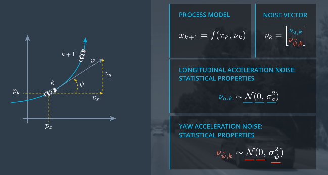
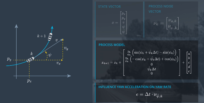
$\nu_{a,k{}}$和$\nu_{\ddot{\psi},k}$ 对于$x$方向位置的影响即(a)是: $\frac{1}{2}(\Delta t)^2 cos(\psi_k) \cdot \nu_{a,k}$
$\nu_{a,k{}}$和$\nu_{\ddot{\psi},k}$ 对于$y$方向位置的影响即(b)是: $\frac{1}{2}(\Delta t)^2 sin(\psi_k) \cdot \nu_{a,k}$
$\nu_{a,k{}}$和$\nu_{\ddot{\psi},k}$ 对于速度的影响即(c)是: $\Large \Delta t \cdot \nu_{a,k}$
$\nu_{a,k{}}$和$\nu_{\ddot{\psi},k}$ 对于偏航角的影响即(d)是: $\Large \frac{1}{2}(\Delta t)^2 \cdot \nu_{\ddot{\psi},k}$
$\nu_{a,k{}}$和$\nu_{\ddot{\psi},k}$ 对于偏航率的影响即(e)是: $\Large \Delta t \cdot \nu_{\ddot{\psi},k}$
3. UKF
3.1 UKF介绍
无味卡尔曼滤波器随时间处理测量值的方式和扩展卡尔曼滤波器是一样的,它们都有预测步骤,这个步骤是独立于测量模型的,在预测步骤,需要使用 CTRV 模型。接下来是更新步骤,我们使用雷达测量模型或激光测量模型,具体取决于我们收到的测量数值类型。也就是说,对于无味卡尔曼滤波器和扩展卡尔曼滤波器可以使用同样的顶层处理链。两者的不同之处是,无味卡尔曼滤波器处理非线性过程模型或测量模型使用的方法叫做无味变换,无味卡尔曼滤波器不需要将非线性函数线性化(不需要像扩展卡尔曼滤波器一样计算雅克比矩阵近似逼近),无味卡尔曼滤波器从高斯分布中提取代表点插入到非线性方程中。
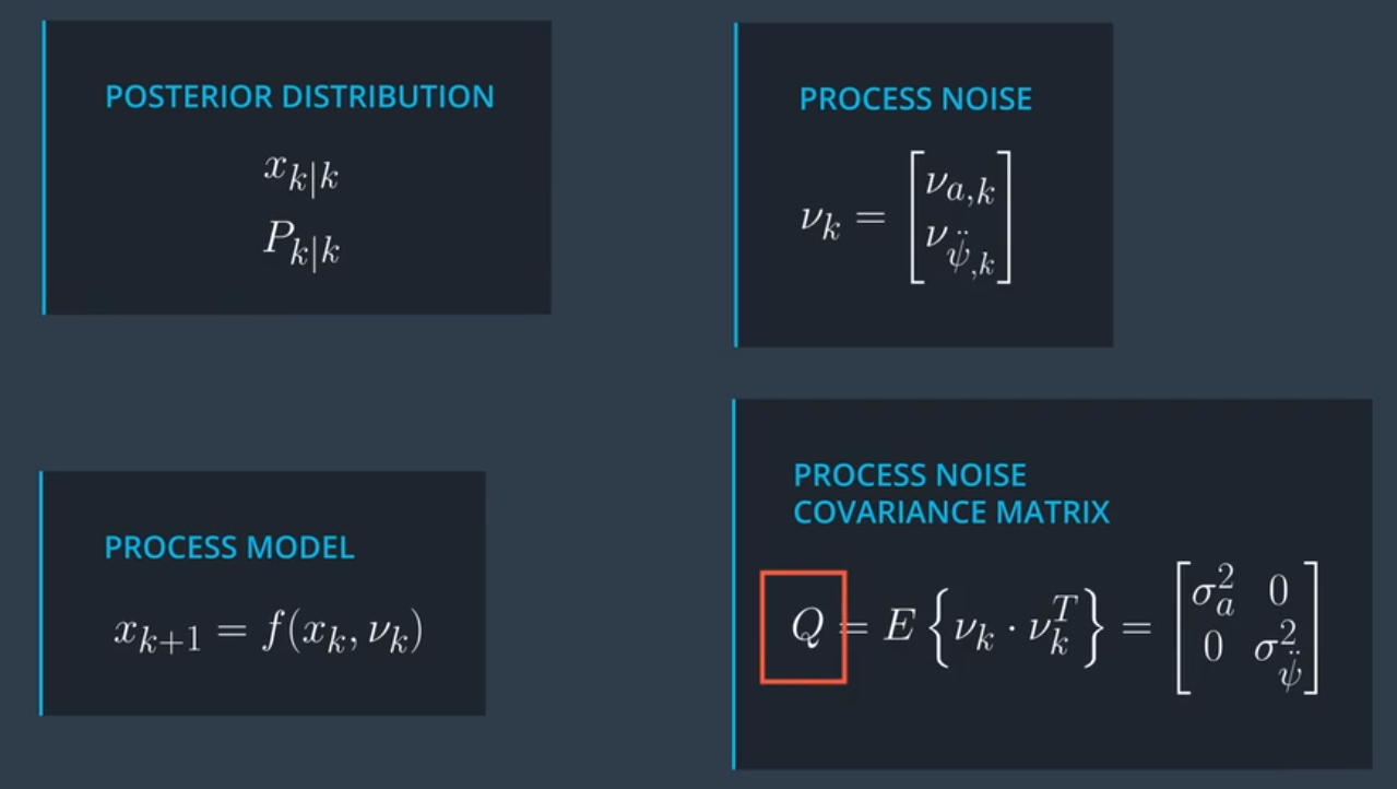
3.2 问题界定
UKF 使用无味变换解决非线性过程模型或非线性测量模型所存在的问题。
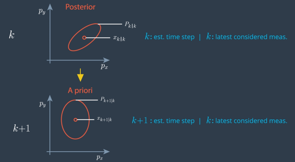
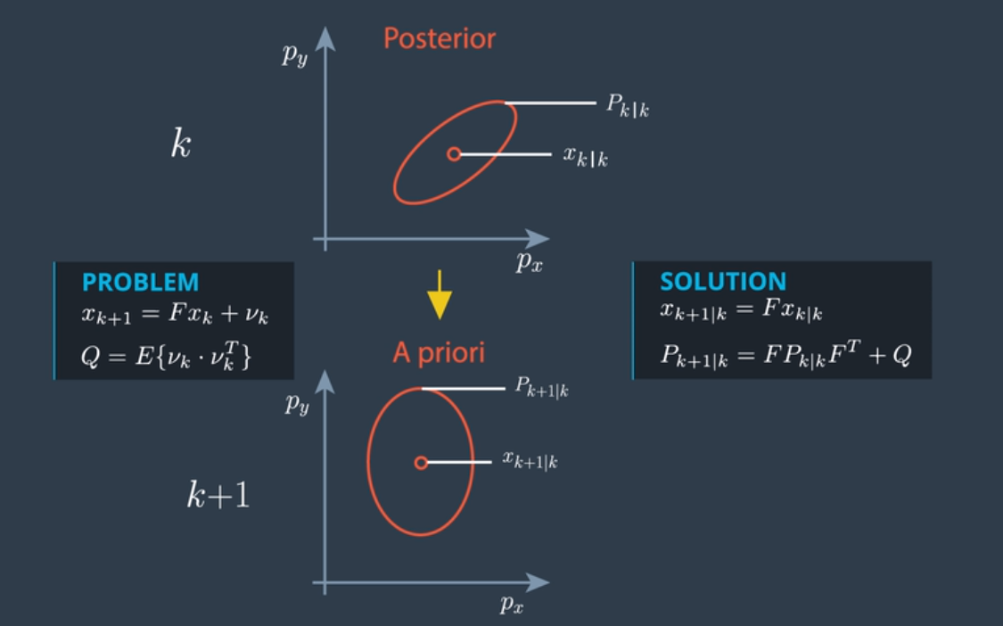
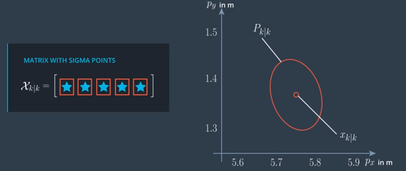
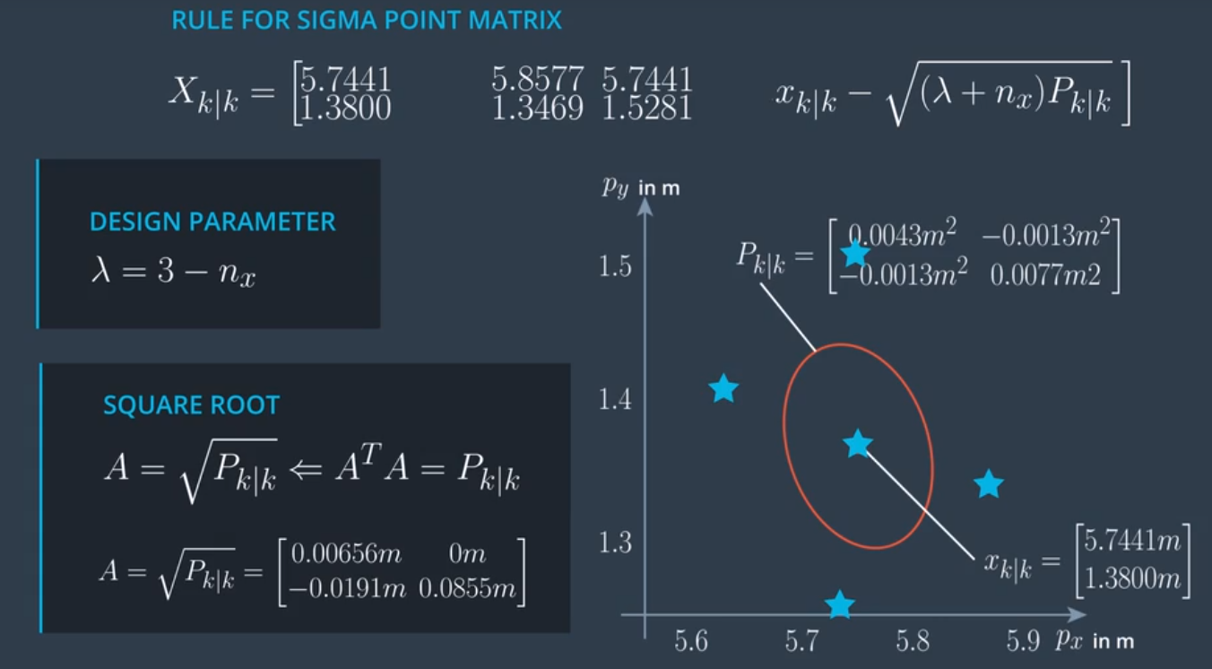
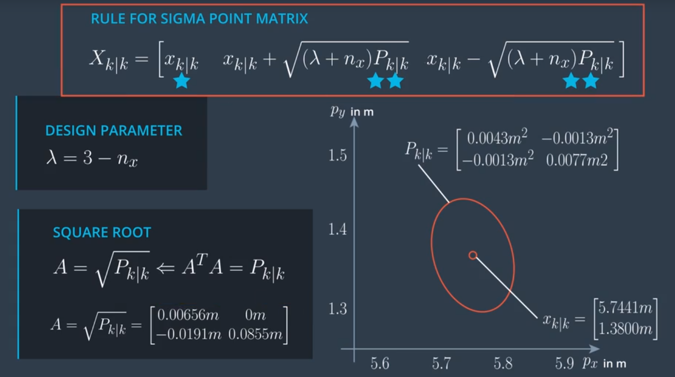
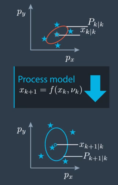
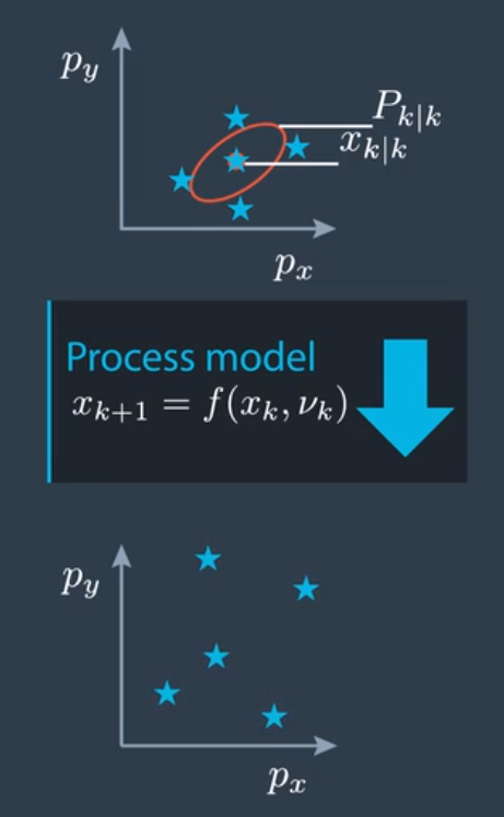
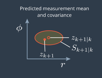
| 假设我们有状态向量均值 x和状态协方差 P 以及时间步 k,我们要做的是预测到时间步 k+1 的均值和协方差。我们有 Xk+1 | k 以及 Pk+1 | k,k | k 表示估算是时间步 k 的,而且时间 k 的测量值已经考虑在内了这也叫做后验估算。k+1 | k 表示估算是时间步 k+1 的,但是最后一个考虑在内的测量值是来自 k 的,这就是预测后的结果,这也叫做先验估算。椭圆描述了不确定性分布,椭圆线上的所有点都有着同样的概率密度。如果不确定性是正态分布的,这些点就呈椭圆形排列,它经常被叫做误差椭圆,可以看作协方差矩阵 P 的可视化。 |
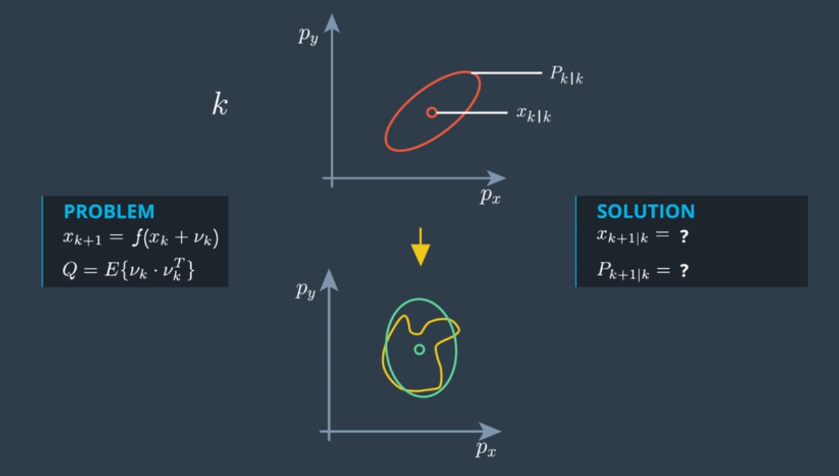
如果过程模型是线性的,则预测问题看起来如上图表示, Q 是过程噪音的协方差矩阵,我们可以使用卡尔曼滤波器求解这个线性预测问题。
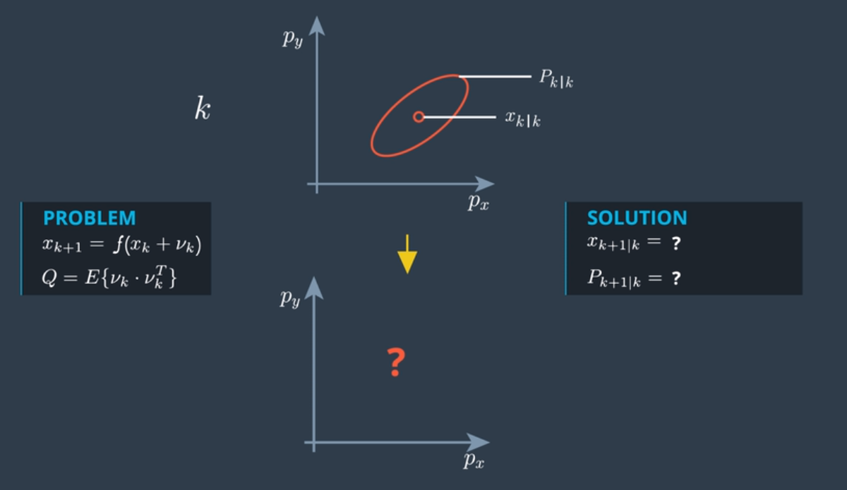
如果过程模型是非线性的,这种情况看起来是怎样的?预测就通过非线性函数 f 定义。
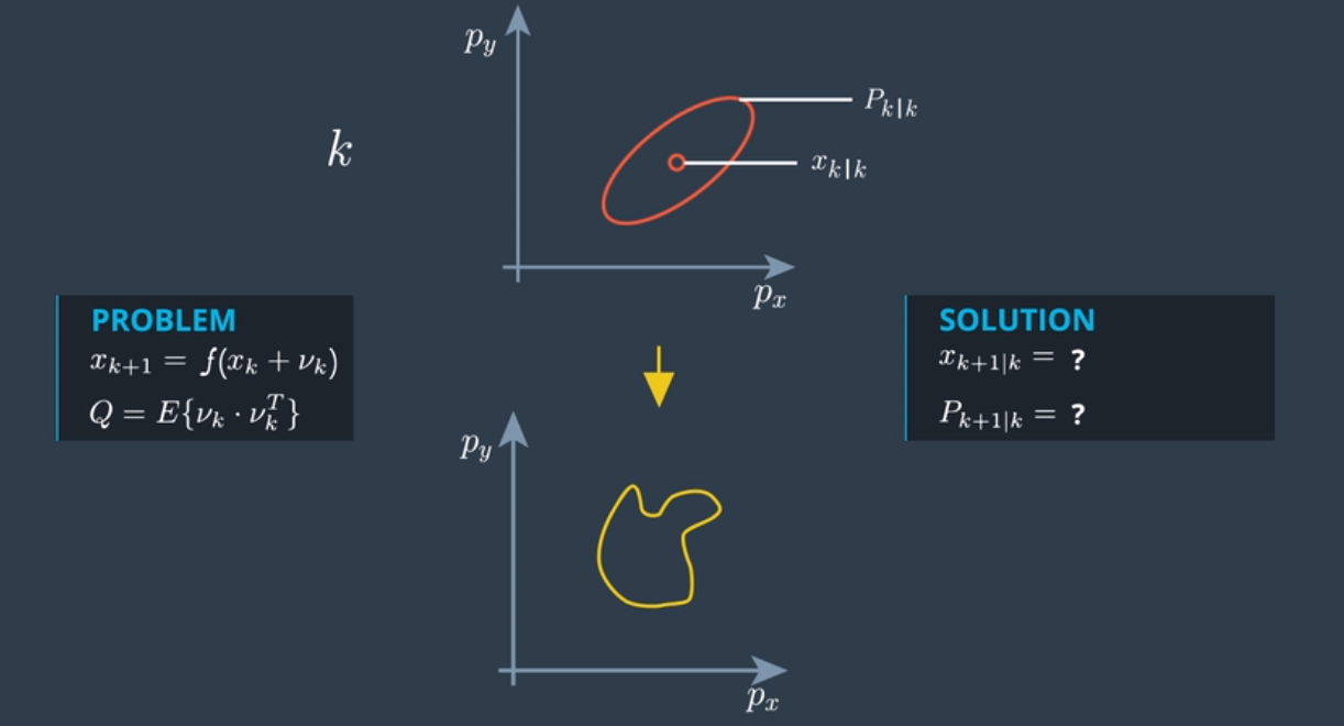
像CTRV这样的非线性过程模型,使用非线性函数预测提供了一个分布,一个通常不再正态的分布,如上图所示。实际上,计算这个预测分布并容易,一般来说只能通过数字计算。粒子滤波器算法算是一种较好的算法来进行这种计算。如上图所示,它将不再是正态分布。
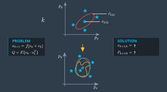
UKF 的原理是把非正态分布的状态分布通过无味变换找出近似的正态分布,也就是说,寻找的是一个均值和协方差矩阵一样的正态分布,尽可能贴近真实预测分布的整体分布,如上图所示。
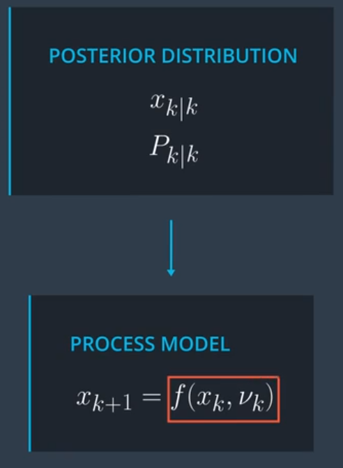
3.3 UKF基本变换
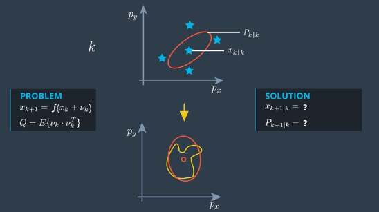
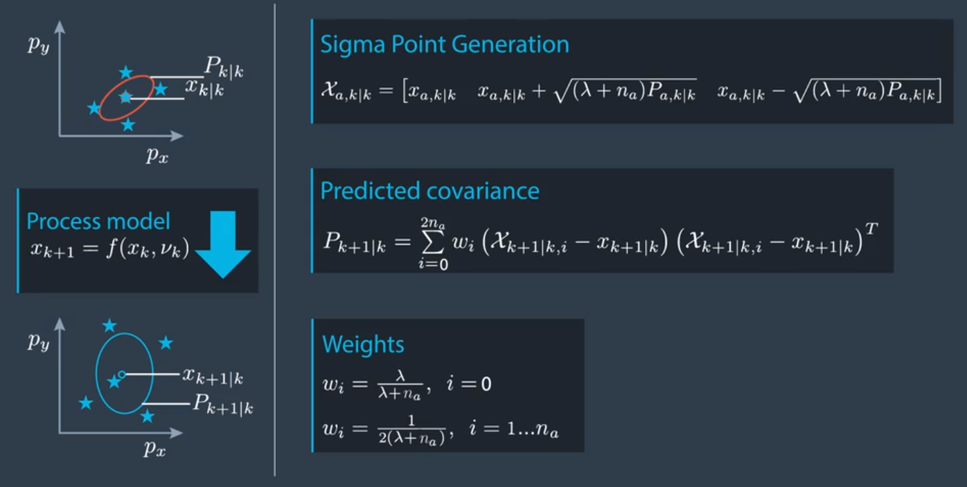
使用非线性函数进行整个状态分布的转换有难度,但使用非线性函数转换状态空间中的单个点非常简单,这就是 sigma点的意义所在。
sigma点分布于状态均值的周围,和每个状态大小的标准偏差的总和(即 sigma)有一定关系,“ sigma点”的命名就是由此而来,它们代表了整个分布。
选择了 sigma点后,只需要把所有单个的 sigma点代入非线性函数 f 即可。这样,它们在预测状态空间的分布就会如上图所示。需要做的只是计算这组 sigma点的均值和协方差。这里的均值和协方差和真正预测的分布近似。
4. UKF完整实现
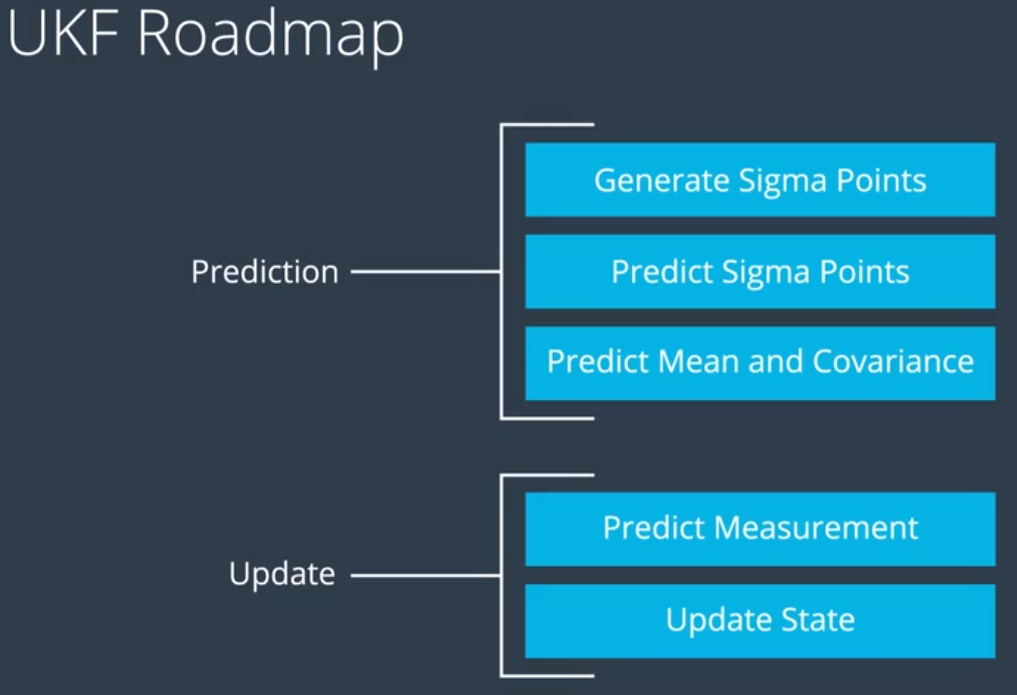
4.1 预测步骤之生成sigma点
4.1.1 以基础状态向量生成sigma点
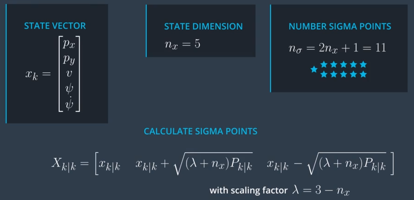
以两个状态向量为例进行说明。
生成sigma点的方程:
\[X_{k|k} = \Bigg [ x_{k|k} \qquad x_{k|k}+\sqrt{(\lambda+n_x)P_{k|k}} \qquad x_{k|k}-\sqrt{(\lambda+n_x)P_{k|k}} \Bigg]\]| $\large x_{k | k}$是sigma矩阵的第一列。 |
| $\large x_{k | k}+\sqrt{(\lambda+n_x)P_{k | k}}$ 是2至 $\large n_x +1$ 列。 |
| $\large x_{k | k}-\sqrt{(\lambda+n_x)P_{k | k}}$ 是 $\large n_x +2$ 至 $\large 2n_x +1$ 列。 |
C++实现生成sigma点矩阵
main.cpp
#include <iostream>
#include "Dense"
#include "ukf.h"

using Eigen::MatrixXd;

int main() {

  // Create a UKF instance
  UKF ukf;

  /**

   * Programming assignment calls
     */
       MatrixXd Xsig = MatrixXd(5, 11);
       ukf.GenerateSigmaPoints(&Xsig);

  // print result
  std::cout << "Xsig = " << std::endl << Xsig << std::endl;

  return 0;
}
ukf.h
#ifndef UKF_H
#define UKF_H

#include "Dense"

class UKF {
 public:
  /**

   * Constructor
     */
       UKF();

  /**

   * Destructor
     */
       virtual ~UKF();

  /**

   * Init Initializes Unscented Kalman filter
     */
       void Init();

  /**

   * assignment functions
     */
       void GenerateSigmaPoints(Eigen::MatrixXd* Xsig_out);
     };

#endif  // UKF_H
ukf.cpp
#include "ukf.h"
#include <iostream>

using Eigen::MatrixXd;
using Eigen::VectorXd;

UKF::UKF() {
  Init();
}

UKF::~UKF() {
}

void UKF::Init() {
}

/**
 * Programming assignment functions:
   */
void UKF::GenerateSigmaPoints(MatrixXd* Xsig_out) {

  // set state dimension
  int n_x = 5;

  // define spreading parameter
  double lambda = 3 - n_x;

  // set example state
  VectorXd x = VectorXd(n_x);
  x <<   5.7441,
         1.3800,
         2.2049,
         0.5015,
         0.3528;

  // set example covariance matrix
  MatrixXd P = MatrixXd(n_x, n_x);
  P <<     0.0043,   -0.0013,    0.0030,   -0.0022,   -0.0020,
          -0.0013,    0.0077,    0.0011,    0.0071,    0.0060,
           0.0030,    0.0011,    0.0054,    0.0007,    0.0008,
          -0.0022,    0.0071,    0.0007,    0.0098,    0.0100,
          -0.0020,    0.0060,    0.0008,    0.0100,    0.0123;

  // create sigma point matrix
  MatrixXd Xsig = MatrixXd(n_x, 2 * n_x + 1);

  // calculate square root of P
  MatrixXd A = P.llt().matrixL();

   // set first column of sigma point matrix
  Xsig.col(0) = x;

  // set remaining sigma points
  for (int i = 0; i < n_x; ++i) {
    Xsig.col(i+1)     = x + sqrt(lambda+n_x) * A.col(i);
    Xsig.col(i+1+n_x) = x - sqrt(lambda+n_x) * A.col(i);
  }

  // print result
  // std::cout << "Xsig = " << std::endl << Xsig << std::endl;

  // write result
  *Xsig_out = Xsig;
}

/**
 * expected result:
 * Xsig =
 * 5.7441  5.85768   5.7441   5.7441   5.7441   5.7441  5.63052   5.7441   5.7441   5.7441   5.7441
 * 1.38  1.34566  1.52806     1.38     1.38     1.38  1.41434  1.23194     1.38     1.38     1.38
 * 2.2049  2.28414  2.24557  2.29582   2.2049   2.2049  2.12566  2.16423  2.11398   2.2049   2.2049
 * 0.5015  0.44339 0.631886 0.516923 0.595227   0.5015  0.55961 0.371114 0.486077 0.407773   0.5015
 * 0.3528 0.299973 0.462123 0.376339  0.48417 0.418721 0.405627 0.243477 0.329261  0.22143 0.286879
   */
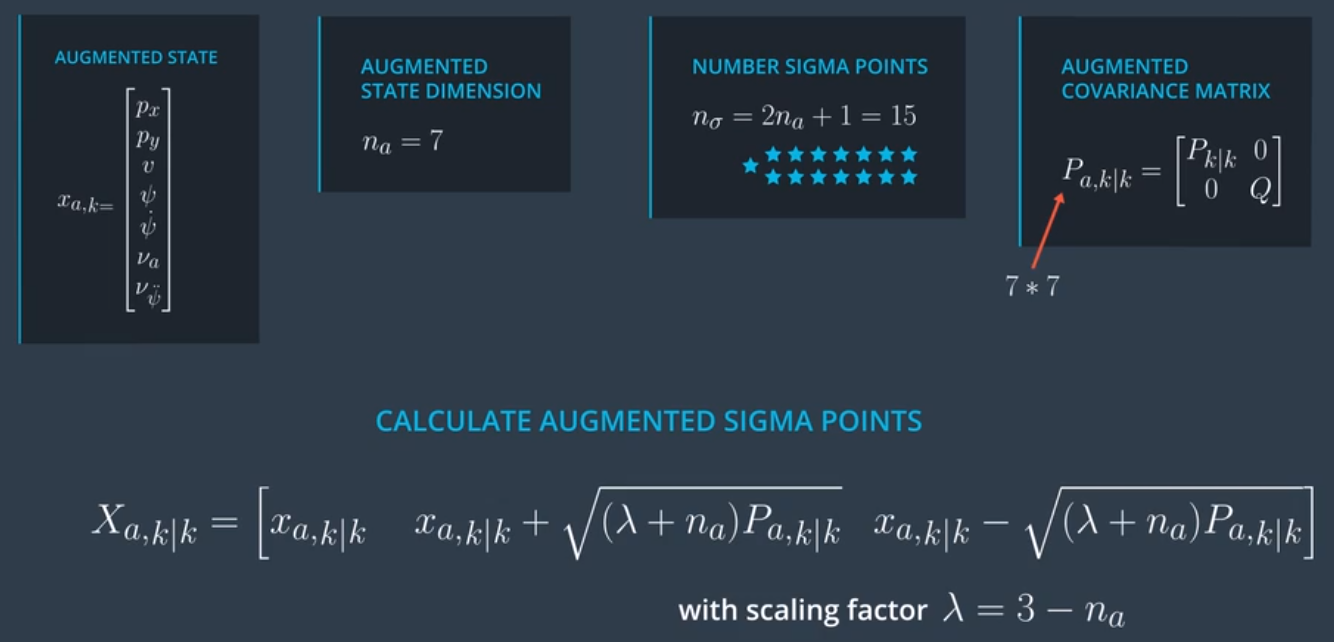
4.1.2 添加过程模型噪音进行sigma点增广
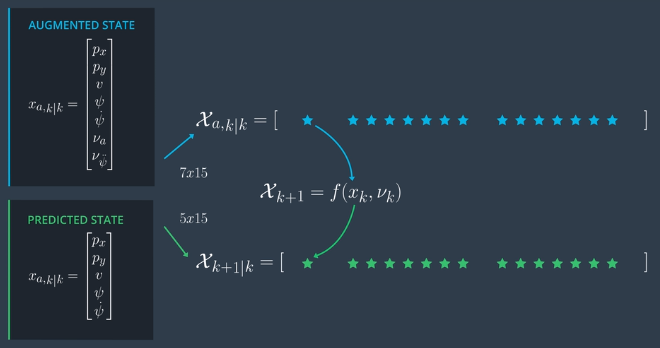
Augmented State =
\[\large x_{a,k} = \begin{bmatrix} p_x\\ p_y\\ v\\ \psi\\ \dot{\psi}\\ \nu_a\\ \nu_{\ddot{\psi}} \end{bmatrix}\]Augmented Covariance Matrix =
\[\large P_{a,k|k} = \begin{bmatrix} P_{k|k} \quad 0 \\ 0 \qquad Q \end{bmatrix}\]C++实现sigma点增广
有用的矩阵和向量函数:
快速将向量y设置为向量x的前n个元素。x.head(n) = y ,其中n是从第一个元素开始的元素个数,y是该大小的输入向量。
快速将矩阵y设置为矩阵x的左上角。x.topLeftCorner(y_size, y_size)
获取矩阵x的平方根,使用函数x.llt().matrixL()
main.cpp
#include "Dense"
#include "ukf.h"

using Eigen::MatrixXd;

int main() {

  // Create a UKF instance
  UKF ukf;

  /**

   * Programming assignment calls
     */
   MatrixXd Xsig_aug = MatrixXd(7, 15);
   ukf.AugmentedSigmaPoints(&Xsig_aug);

  return 0;
}
ukf.h
#ifndef UKF_H
#define UKF_H

#include "Dense"

class UKF {
 public:
  /**

   * Constructor
     */
       UKF();

  /**
   * Destructor
     */
       virtual ~UKF();
  /**
   * Init Initializes Unscented Kalman filter
     */
       void Init();
  /**

   * assignment functions
     */
       void AugmentedSigmaPoints(Eigen::MatrixXd* Xsig_out);
     };

#endif  // UKF_H
ukf.cpp
#include <iostream>
#include "ukf.h"

using Eigen::MatrixXd;
using Eigen::VectorXd;

UKF::UKF() {
  Init();
}

UKF::~UKF() {

}

void UKF::Init() {

}

/**

 * Programming assignment functions:
   */

void UKF::AugmentedSigmaPoints(MatrixXd* Xsig_out) {

  // set state dimension
  int n_x = 5;

  // set augmented dimension
  int n_aug = 7;

  // Process noise standard deviation longitudinal acceleration in m/s^2
  double std_a = 0.2;

  // Process noise standard deviation yaw acceleration in rad/s^2
  double std_yawdd = 0.2;

  // define spreading parameter
  double lambda = 3 - n_aug;

  // set example state
  VectorXd x = VectorXd(n_x);
  x <<   5.7441,
         1.3800,
         2.2049,
         0.5015,
         0.3528;

  // create example covariance matrix
  MatrixXd P = MatrixXd(n_x, n_x);
  P <<     0.0043,   -0.0013,    0.0030,   -0.0022,   -0.0020,
          -0.0013,    0.0077,    0.0011,    0.0071,    0.0060,
           0.0030,    0.0011,    0.0054,    0.0007,    0.0008,
          -0.0022,    0.0071,    0.0007,    0.0098,    0.0100,
          -0.0020,    0.0060,    0.0008,    0.0100,    0.0123;

  // create augmented mean vector
  VectorXd x_aug = VectorXd(7);

  // create augmented state covariance
  MatrixXd P_aug = MatrixXd(7, 7);

  // create sigma point matrix
  MatrixXd Xsig_aug = MatrixXd(n_aug, 2 * n_aug + 1);

  // create augmented mean state
  // 在基础状态均值上加两个噪声值。噪声值的平均值为零,将这些数字设置为零。
  x_aug.head(5) = x;
  x_aug(5) = 0;
  x_aug(6) = 0;

  // create augmented covariance matrix
  // 用零填充增广协方差矩阵。用函数topLeftcorner设置增广协方差矩阵的左上角块为P。
  // 手动把矩阵Q放入增广协方差矩阵的右下部分(即矩阵的第6行第6列\sigma_a^2和第7行第7列为\sigma_{\ddot{\psi}}^2 .
  P_aug.fill(0.0);
  P_aug.topLeftCorner(5,5) = P;
  P_aug(5,5) = std_a*std_a;
  P_aug(6,6) = std_yawdd*std_yawdd;

  // create square root matrix
  MatrixXd L = P_aug.llt().matrixL();

  // create augmented sigma points
  Xsig_aug.col(0)  = x_aug;
  for (int i = 0; i< n_aug; ++i) {
    Xsig_aug.col(i+1)       = x_aug + sqrt(lambda+n_aug) * L.col(i);
    Xsig_aug.col(i+1+n_aug) = x_aug - sqrt(lambda+n_aug) * L.col(i);
  }

  // print result
  std::cout << "Xsig_aug = " << std::endl << Xsig_aug << std::endl;

  // write result
  *Xsig_out = Xsig_aug;
}

/**
 * expected result:
 * Xsig_aug =
 * 5.7441  5.85768   5.7441   5.7441   5.7441   5.7441   5.7441   5.7441  5.63052   5.7441   5.7441   5.7441   5.7441   5.7441   5.7441
 * 1.38  1.34566  1.52806     1.38     1.38     1.38     1.38     1.38  1.41434  1.23194     1.38     1.38     1.38     1.38     1.38
 * 2.2049  2.28414  2.24557  2.29582   2.2049   2.2049   2.2049   2.2049  2.12566  2.16423  2.11398   2.2049   2.2049   2.2049   2.2049
 * 0.5015  0.44339 0.631886 0.516923 0.595227   0.5015   0.5015   0.5015  0.55961 0.371114 0.486077 0.407773   0.5015   0.5015   0.5015
 * 0.3528 0.299973 0.462123 0.376339  0.48417 0.418721   0.3528   0.3528 0.405627 0.243477 0.329261  0.22143 0.286879   0.3528   0.3528
 * 0        0        0        0        0        0  0.34641        0        0        0        0        0        0 -0.34641        0
 * 0        0        0        0        0        0        0  0.34641        0        0        0        0        0        0 -0.34641
    */
4.2 预测步骤之sigma点位置预测
有用的方程式:
\[x = \begin{bmatrix} p_x \\ p_y \\ v \\ \psi \\ \dot{\psi} \end{bmatrix}\]当$\large \dot{\psi}_k$不等于0:
\[\text{State}= x_{k+1} = x_k + \begin{bmatrix} \frac{v_k}{\dot{\psi}_k}(sin(\psi_k+\dot{\psi}_k\Delta t )-sin(\psi_k))\\ \frac{v_k}{\dot{\psi}_k}(-cos(\psi_k+\dot{\psi}_k\Delta t )+cos(\psi_k))\\ 0\\ \dot{\psi}_k\Delta t\\ 0 \end{bmatrix} +\begin{bmatrix} \frac{1}{2}(\Delta t)^2cos(\psi_k)\nu_{a,k}\\ \frac{1}{2}(\Delta t)^2sin(\psi_k)\nu_{a,k}\\ \Delta t\cdot\nu_{a,k}\\ \frac{1}{2}(\Delta t)^2\nu_{\ddot{\psi},k}\\ \Delta t\cdot\nu_{\ddot{\psi},k} \end{bmatrix}\]当$\large \dot{\psi}_k$等于0:
\[\text{State} =x_{k+1} = x_k + \begin{bmatrix} v_kcos(\psi_k)\Delta t\\ v_ksin(\psi_k)\Delta t\\ 0\\ \dot{\psi}_k\Delta t\\ 0 \end{bmatrix} +\begin{bmatrix} \frac{1}{2}(\Delta t)^2cos(\psi_k)\nu_{a,k}\\ \frac{1}{2}(\Delta t)^2sin(\psi_k)\nu_{a,k}\\ \Delta t\cdot\nu_{a,k}\\ \frac{1}{2}(\Delta t)^2\nu_{\ddot{\psi},k}\\ \Delta t\cdot\nu_{\ddot{\psi},k} \end{bmatrix}\]当$\large \dot{\psi_k} = 0$,则$\large \dot{\psi_k}\Delta{t}$也等于0。
C++实现sigma点预测
main.cpp
#include "Dense"
#include "ukf.h"

using Eigen::MatrixXd;

int main() {

  // Create a UKF instance
  UKF ukf;

  /**

   * Programming assignment calls
     */
       MatrixXd Xsig_pred = MatrixXd(15, 5);
       ukf.SigmaPointPrediction(&Xsig_pred);

  return 0;
}
ukf.h
#ifndef UKF_H
#define UKF_H

#include "Dense"

class UKF {
 public:
  /**

   * Constructor
     */
       UKF();

  /**

   * Destructor
     */
       virtual ~UKF();

  /**

   * Init Initializes Unscented Kalman filter
     */
       void Init();

  /**

   * assignment functions
     */
       void SigmaPointPrediction(Eigen::MatrixXd* Xsig_out);
     };

#endif  // UKF_H
ukf.cpp
#include <iostream>
#include "ukf.h"

using Eigen::MatrixXd;
using Eigen::VectorXd;

UKF::UKF() {
  Init();
}

UKF::~UKF() {

}

void UKF::Init() {

}

/**

 * Programming assignment functions:
   */

void UKF::SigmaPointPrediction(MatrixXd* Xsig_out) {

  // set state dimension
  int n_x = 5;

  // set augmented dimension
  int n_aug = 7;

  // create example sigma point matrix
  MatrixXd Xsig_aug = MatrixXd(n_aug, 2 * n_aug + 1);
  Xsig_aug <<
    5.7441,  5.85768,   5.7441,   5.7441,   5.7441,   5.7441,   5.7441,   5.7441,   5.63052,   5.7441,   5.7441,   5.7441,   5.7441,   5.7441,   5.7441,
      1.38,  1.34566,  1.52806,     1.38,     1.38,     1.38,     1.38,     1.38,   1.41434,  1.23194,     1.38,     1.38,     1.38,     1.38,     1.38,
    2.2049,  2.28414,  2.24557,  2.29582,   2.2049,   2.2049,   2.2049,   2.2049,   2.12566,  2.16423,  2.11398,   2.2049,   2.2049,   2.2049,   2.2049,
    0.5015,  0.44339, 0.631886, 0.516923, 0.595227,   0.5015,   0.5015,   0.5015,   0.55961, 0.371114, 0.486077, 0.407773,   0.5015,   0.5015,   0.5015,
    0.3528, 0.299973, 0.462123, 0.376339,  0.48417, 0.418721,   0.3528,   0.3528,  0.405627, 0.243477, 0.329261,  0.22143, 0.286879,   0.3528,   0.3528,
         0,        0,        0,        0,        0,        0,  0.34641,        0,         0,        0,        0,        0,        0, -0.34641,        0,
         0,        0,        0,        0,        0,        0,        0,  0.34641,         0,        0,        0,        0,        0,        0, -0.34641;

  // create matrix with predicted sigma points as columns
  MatrixXd Xsig_pred = MatrixXd(n_x, 2 * n_aug + 1);

  double delta_t = 0.1; // time diff in sec

  // predict sigma points
  for (int i = 0; i< 2*n_aug+1; ++i) {
    // extract values for better readability
    double p_x = Xsig_aug(0,i);
    double p_y = Xsig_aug(1,i);
    double v = Xsig_aug(2,i);
    double yaw = Xsig_aug(3,i);
    double yawd = Xsig_aug(4,i);
    double nu_a = Xsig_aug(5,i);
    double nu_yawdd = Xsig_aug(6,i);

    // predicted state values
    double px_p, py_p;

    // avoid division by zero
    if (fabs(yawd) > 0.001) {
        px_p = p_x + v/yawd * ( sin (yaw + yawd*delta_t) - sin(yaw));
        py_p = p_y + v/yawd * ( cos(yaw) - cos(yaw+yawd*delta_t) );
    } else {
        px_p = p_x + v*delta_t*cos(yaw);
        py_p = p_y + v*delta_t*sin(yaw);
    }

    double v_p = v;
    double yaw_p = yaw + yawd*delta_t;
    double yawd_p = yawd;

    // add noise
    px_p = px_p + 0.5*nu_a*delta_t*delta_t * cos(yaw);
    py_p = py_p + 0.5*nu_a*delta_t*delta_t * sin(yaw);
    v_p = v_p + nu_a*delta_t;

    yaw_p = yaw_p + 0.5*nu_yawdd*delta_t*delta_t;
    yawd_p = yawd_p + nu_yawdd*delta_t;

    // write predicted sigma point into right column
    Xsig_pred(0,i) = px_p;
    Xsig_pred(1,i) = py_p;
    Xsig_pred(2,i) = v_p;
    Xsig_pred(3,i) = yaw_p;
    Xsig_pred(4,i) = yawd_p;

  }

  // print result
  std::cout << "Xsig_pred = " << std::endl << Xsig_pred << std::endl;

  // write result
  *Xsig_out = Xsig_pred;
}
/**
* expected result:
* Xsig_pred =
* 5.93553 6.06251 5.92217 5.9415 5.92361 5.93516 5.93705 5.93553 5.80832 5.94481 5.92935 5.94553 5.93589 5.93401 5.93553
* 1.48939 1.44673 1.66484 1.49719 1.508 1.49001 1.49022 1.48939 1.5308 1.31287 1.48182 1.46967 1.48876 1.48855 1.48939
* 2.2049 2.28414 2.24557 2.29582 2.2049 2.2049 2.23954 2.2049 2.12566 2.16423 2.11398 2.2049 2.2049 2.17026 2.2049
* 0.53678 0.473387 0.678098 0.554557 0.643644 0.543372 0.53678 0.538512 0.600173 0.395462 0.519003 0.429916 0.530188 0.53678 0.535048
* 0.3528 0.299973 0.462123 0.376339 0.48417 0.418721 0.3528 0.387441 0.405627 0.243477 0.329261 0.22143 0.286879 0.3528 0.318159
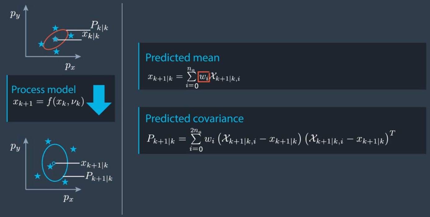
4.3 预测步骤之根据预测的sigma点计算整体预测的均值和协方差
有用的方程式:
- Weights
- Predicted Mean
- Predicted Covariance
C++实现根据预测的sigma点计算整体预测均值和协方差
main.cpp
#include "Dense"
#include "ukf.h"

using Eigen::MatrixXd;
using Eigen::VectorXd;

int main() {

  // Create a UKF instance
  UKF ukf;

  /**

   * Programming assignment calls
     */
       VectorXd x_pred = VectorXd(5);
       MatrixXd P_pred = MatrixXd(5, 5);
       ukf.PredictMeanAndCovariance(&x_pred, &P_pred);

  return 0;
}
ukf.h
#ifndef UKF_H
#define UKF_H

#include "Dense"

class UKF {
 public:
  /**
   * Constructor
     */
       UKF();

  /**
   * Destructor
     */
       virtual ~UKF();

  /**
   * Init Initializes Unscented Kalman filter
     */
       void Init();

  /**
   * Student assignment functions
     */
       void PredictMeanAndCovariance(Eigen::VectorXd* x_pred,
                             Eigen::MatrixXd* P_pred);
     };

#endif  // UKF_H
ukf.cpp
#include <iostream>
#include "ukf.h"

using Eigen::MatrixXd;
using Eigen::VectorXd;

UKF::UKF() {
  Init();
}

UKF::~UKF() {

}

void UKF::Init() {

}

/**
 * Programming assignment functions:
   */

void UKF::PredictMeanAndCovariance(VectorXd* x_out, MatrixXd* P_out) {

  // set state dimension
  int n_x = 5;

  // set augmented dimension
  int n_aug = 7;

  // define spreading parameter
  double lambda = 3 - n_aug;

  // create example matrix with predicted sigma points
  MatrixXd Xsig_pred = MatrixXd(n_x, 2 * n_aug + 1);
  Xsig_pred <<
         5.9374,  6.0640,   5.925,  5.9436,  5.9266,  5.9374,  5.9389,  5.9374,  5.8106,  5.9457,  5.9310,  5.9465,  5.9374,  5.9359,  5.93744,
           1.48,  1.4436,   1.660,  1.4934,  1.5036,    1.48,  1.4868,    1.48,  1.5271,  1.3104,  1.4787,  1.4674,    1.48,  1.4851,    1.486,
          2.204,  2.2841,  2.2455,  2.2958,   2.204,   2.204,  2.2395,   2.204,  2.1256,  2.1642,  2.1139,   2.204,   2.204,  2.1702,   2.2049,
         0.5367, 0.47338, 0.67809, 0.55455, 0.64364, 0.54337,  0.5367, 0.53851, 0.60017, 0.39546, 0.51900, 0.42991, 0.530188,  0.5367, 0.535048,
          0.352, 0.29997, 0.46212, 0.37633,  0.4841, 0.41872,   0.352, 0.38744, 0.40562, 0.24347, 0.32926,  0.2214, 0.28687,   0.352, 0.318159;

  // create vector for weights
  VectorXd weights = VectorXd(2*n_aug+1);

  // create vector for predicted state
  VectorXd x = VectorXd(n_x);

  // create covariance matrix for prediction
  MatrixXd P = MatrixXd(n_x, n_x);

  // set weights
  double weight_0 = lambda/(lambda+n_aug);
  weights(0) = weight_0;
  for (int i=1; i<2*n_aug+1; ++i) {  // 2n+1 weights
    double weight = 0.5/(n_aug+lambda);
    weights(i) = weight;
  }

  // predict state mean
  x.fill(0.0);
  for (int i = 0; i < 2 * n_aug + 1; ++i) {  // iterate over sigma points
    x = x + weights(i) * Xsig_pred.col(i);
  }

  // predict state covariance matrix
  P.fill(0.0);
  for (int i = 0; i < 2 * n_aug + 1; ++i) {  // iterate over sigma points
    // state difference
    VectorXd x_diff = Xsig_pred.col(i) - x;
    // angle normalization
    while (x_diff(3)> M_PI) x_diff(3)-=2.*M_PI;
    while (x_diff(3)<-M_PI) x_diff(3)+=2.*M_PI;

    P = P + weights(i) * x_diff * x_diff.transpose() ;
  }

  // print result
  std::cout << "Predicted state" << std::endl;
  std::cout << x << std::endl;
  std::cout << "Predicted covariance matrix" << std::endl;
  std::cout << P << std::endl;

  // write result
  *x_out = x;
  *P_out = P;
}

/**
* expected result x:
* x =
5.93637
1.49035
2.20528
0.536853
0.353577

* expected result p:
* P =
0.00543425 -0.0024053 0.00341576 -0.00348196 -0.00299378
-0.0024053 0.010845 0.0014923 0.00980182 0.00791091
0.00341576 0.0014923 0.00580129 0.000778632 0.000792973
-0.00348196 0.00980182 0.000778632 0.0119238 0.0112491
-0.00299378 0.00791091 0.000792973 0.0112491 0.0126972
4.4 更新步骤之测量分布预测
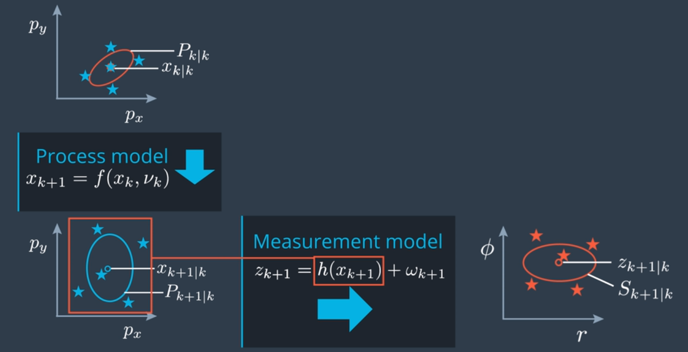
在更新步骤,需把预测状态转换为测量空间,定义无味变换的函数叫做测量模型。当然,我们现在必须考虑是哪种传感器生成了当前测量值,并使用对应的测量模型。我们这里的问题和我们在预测步骤碰到的问题非常类似,我们需要通过非线性函数来转换一个分布,这样我们就能和之前的状态预测一样,在中心变换中应用同样的函数。
但是,我们这里有两个捷径,可以更简单一些。可以跳过生成 sigma点和增广sigma点,只需重用我们在预测步骤已经有的 sigma点即可,因为虽然这里的测量模型(雷达测量模型)是非线性函数,但其测量噪音具备单纯的累加效果,所以也可以跳过在预测步骤处理过程噪音的增广sigma点步骤。
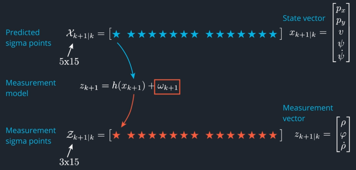
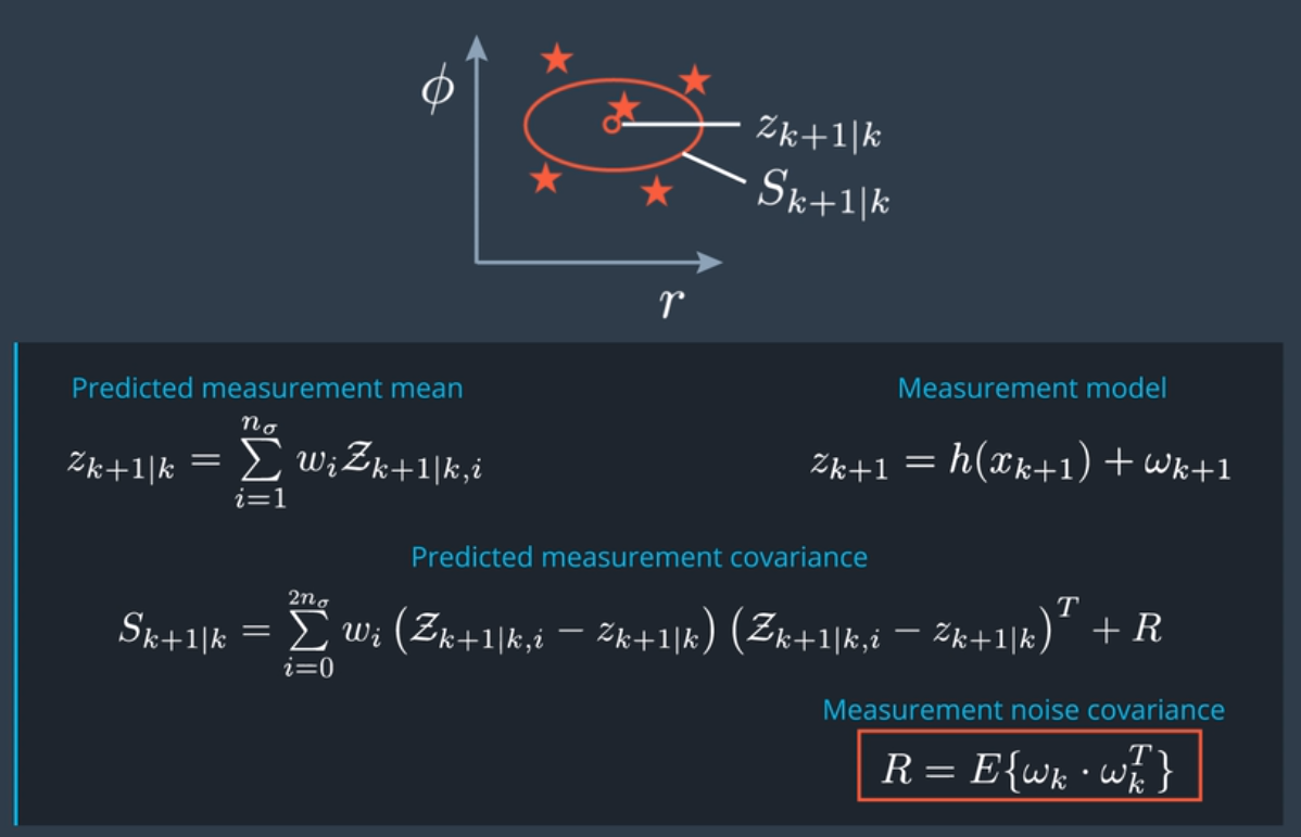
在更新步骤预测测量分布时只需要把预测步骤里的sigma点转换为测量空间,并使用这些点来计算预测测量值的均值和协方差矩阵。转换后的测量 sigma点,存储为矩阵中的列。

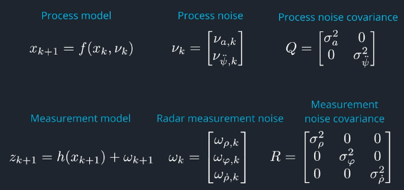
有用的方程式
- State Vector
- Measurement Vector
- Measurement Model
- Predicted Measurement Mean
- Predicted Covariance
C++实现更新步骤之测量分布预测
main.cpp
#include "Dense"
#include "ukf.h"

using Eigen::MatrixXd;
using Eigen::VectorXd;

int main() {

  // Create a UKF instance
  UKF ukf;

  /**
   * Programming assignment calls
     */
   VectorXd z_out = VectorXd(3);
   MatrixXd S_out = MatrixXd(3, 3);
   ukf.PredictRadarMeasurement(&z_out, &S_out);

  return 0;
}
ukf.h
#ifndef UKF_H
#define UKF_H

#include "Dense"

class UKF {
 public:
  /**
   * Constructor
     */
       UKF();

  /**
   * Destructor
     */
       virtual ~UKF();

  /**
   * Init Initializes Unscented Kalman filter
     */
       void Init();

  /**
   * assignment functions
     */
       void PredictRadarMeasurement(Eigen::VectorXd* z_out,
                            Eigen::MatrixXd* S_out);
     };

#endif  // UKF_H
ukf.cpp
#include <iostream>
#include "ukf.h"

using Eigen::MatrixXd;
using Eigen::VectorXd;

UKF::UKF() {
  Init();
}

UKF::~UKF() {

}

void UKF::Init() {

}

/**
 * Programming assignment functions:
   */

void UKF::PredictRadarMeasurement(VectorXd* z_out, MatrixXd* S_out) {

  // set state dimension
  int n_x = 5;

  // set augmented dimension
  int n_aug = 7;

  // set measurement dimension, radar can measure r, phi, and r_dot
  int n_z = 3;

  // define spreading parameter
  double lambda = 3 - n_aug;

  // set vector for weights
  VectorXd weights = VectorXd(2*n_aug+1);
  double weight_0 = lambda/(lambda+n_aug);
  double weight = 0.5/(lambda+n_aug);
  weights(0) = weight_0;

  for (int i=1; i<2*n_aug+1; ++i) {
    weights(i) = weight;
  }

  // radar measurement noise standard deviation radius in m
  double std_radr = 0.3;

  // radar measurement noise standard deviation angle in rad
  double std_radphi = 0.0175;

  // radar measurement noise standard deviation radius change in m/s
  double std_radrd = 0.1;

  // create example matrix with predicted sigma points
  MatrixXd Xsig_pred = MatrixXd(n_x, 2 * n_aug + 1);
  Xsig_pred <<
         5.9374,  6.0640,   5.925,  5.9436,  5.9266,  5.9374,  5.9389,  5.9374,  5.8106,  5.9457,  5.9310,  5.9465,  5.9374,  5.9359,  5.93744,
           1.48,  1.4436,   1.660,  1.4934,  1.5036,    1.48,  1.4868,    1.48,  1.5271,  1.3104,  1.4787,  1.4674,    1.48,  1.4851,    1.486,
          2.204,  2.2841,  2.2455,  2.2958,   2.204,   2.204,  2.2395,   2.204,  2.1256,  2.1642,  2.1139,   2.204,   2.204,  2.1702,   2.2049,
         0.5367, 0.47338, 0.67809, 0.55455, 0.64364, 0.54337,  0.5367, 0.53851, 0.60017, 0.39546, 0.51900, 0.42991, 0.530188,  0.5367, 0.535048,
          0.352, 0.29997, 0.46212, 0.37633,  0.4841, 0.41872,   0.352, 0.38744, 0.40562, 0.24347, 0.32926,  0.2214, 0.28687,   0.352, 0.318159;

  // create matrix for sigma points in measurement space
  MatrixXd Zsig = MatrixXd(n_z, 2 * n_aug + 1);

  // mean predicted measurement
  VectorXd z_pred = VectorXd(n_z);

  // measurement covariance matrix S
  MatrixXd S = MatrixXd(n_z,n_z);

  // transform sigma points into measurement space
  for (int i = 0; i < 2 * n_aug + 1; ++i) {  // 2n+1 simga points
    // extract values for better readability
    double p_x = Xsig_pred(0,i);
    double p_y = Xsig_pred(1,i);
    double v  = Xsig_pred(2,i);
    double yaw = Xsig_pred(3,i);

    double v1 = cos(yaw)*v;
    double v2 = sin(yaw)*v;

    // measurement model
    Zsig(0,i) = sqrt(p_x*p_x + p_y*p_y);                       // r
    Zsig(1,i) = atan2(p_y,p_x);                                // phi
    Zsig(2,i) = (p_x*v1 + p_y*v2) / sqrt(p_x*p_x + p_y*p_y);   // r_dot

  }

  // mean predicted measurement
  z_pred.fill(0.0);
  for (int i=0; i < 2*n_aug+1; ++i) {
    z_pred = z_pred + weights(i) * Zsig.col(i);
  }

  // innovation covariance matrix S
  S.fill(0.0);
  for (int i = 0; i < 2 * n_aug + 1; ++i) {  // 2n+1 simga points
    // residual
    VectorXd z_diff = Zsig.col(i) - z_pred;

    // angle normalization
    while (z_diff(1)> M_PI) z_diff(1)-=2.*M_PI;
    while (z_diff(1)<-M_PI) z_diff(1)+=2.*M_PI;

    S = S + weights(i) * z_diff * z_diff.transpose();

  }

  // add measurement noise covariance matrix
  MatrixXd R = MatrixXd(n_z,n_z);
  R <<  std_radr*std_radr, 0, 0,
        0, std_radphi*std_radphi, 0,
        0, 0,std_radrd*std_radrd;
  S = S + R;

  // print result
  std::cout << "z_pred: " << std::endl << z_pred << std::endl;
  std::cout << "S: " << std::endl << S << std::endl;

  // write result
  *z_out = z_pred;
  *S_out = S;
}

/**
* expected result z_out:
* z_pred =
6.12155
0.245993
2.10313
* expected result s_out:
* S =
0.0946171 -0.000139448 0.00407016
-0.000139448 0.000617548 -0.000770652
0.00407016 -0.000770652 0.0180917
4.5 更新步骤之状态更新
有预测的状态均值和协方差以及预测的测量均值和协方差。当时间步 k+1 收到实际测量值 z_k+1,就可以像标准卡尔曼滤波器一样生成更新的状态均值和更新的状态协方差矩阵。
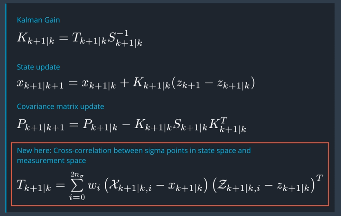
与标准卡尔曼滤波器的区别在于如何计算卡尔曼增益 K,在这里需要状态空间的预测 sigma点和测量空间中的预测 sigma点之间的互相关联矩阵。
有用的方程式
- Cross-correlation Matrix
- Kalman gain K
- Update State
- Covariance Matrix Update
C++实现UKF状态更新
main.cpp
#include "Dense"
#include "ukf.h"

using Eigen::MatrixXd;
using Eigen::VectorXd;

int main() {

  // Create a UKF instance
  UKF ukf;

  /**

   * Programming assignment calls
     */
       VectorXd x_out = VectorXd(5);
       MatrixXd P_out = MatrixXd(5, 5);
       ukf.UpdateState(&x_out, &P_out);

  return 0;
}
ukf.h
#ifndef UKF_H
#define UKF_H

#include "Dense"

class UKF {
 public:
  /**
   * Constructor
     */
       UKF();

  /**
   * Destructor
     */
       virtual ~UKF();

  /**
   * Init Initializes Unscented Kalman filter
     */
       void Init();

  /**
   * Student assignment functions
     */
       void UpdateState(Eigen::VectorXd* x_out,
                Eigen::MatrixXd* P_out);
     };

#endif  // UKF_H
ukf.cpp
#include <iostream>
#include "ukf.h"

using Eigen::MatrixXd;
using Eigen::VectorXd;

UKF::UKF() {
  Init();
}

UKF::~UKF() {
}

void UKF::Init() {

}

/**

 * Programming assignment functions:
   */

void UKF::UpdateState(VectorXd* x_out, MatrixXd* P_out) {

  // set state dimension
  int n_x = 5;

  // set augmented dimension
  int n_aug = 7;

  // set measurement dimension, radar can measure r, phi, and r_dot
  int n_z = 3;

  // define spreading parameter
  double lambda = 3 - n_aug;

  // set vector for weights
  VectorXd weights = VectorXd(2*n_aug+1);
  double weight_0 = lambda/(lambda+n_aug);
  double weight = 0.5/(lambda+n_aug);
  weights(0) = weight_0;

  for (int i=1; i<2*n_aug+1; ++i) {
    weights(i) = weight;
  }

  // create example matrix with predicted sigma points in state space
  MatrixXd Xsig_pred = MatrixXd(n_x, 2 * n_aug + 1);
  Xsig_pred <<
     5.9374,  6.0640,   5.925,  5.9436,  5.9266,  5.9374,  5.9389,  5.9374,  5.8106,  5.9457,  5.9310,  5.9465,  5.9374,  5.9359,  5.93744,
       1.48,  1.4436,   1.660,  1.4934,  1.5036,    1.48,  1.4868,    1.48,  1.5271,  1.3104,  1.4787,  1.4674,    1.48,  1.4851,    1.486,
      2.204,  2.2841,  2.2455,  2.2958,   2.204,   2.204,  2.2395,   2.204,  2.1256,  2.1642,  2.1139,   2.204,   2.204,  2.1702,   2.2049,
     0.5367, 0.47338, 0.67809, 0.55455, 0.64364, 0.54337,  0.5367, 0.53851, 0.60017, 0.39546, 0.51900, 0.42991, 0.530188,  0.5367, 0.535048,
      0.352, 0.29997, 0.46212, 0.37633,  0.4841, 0.41872,   0.352, 0.38744, 0.40562, 0.24347, 0.32926,  0.2214, 0.28687,   0.352, 0.318159;

  // create example vector for predicted state mean
  VectorXd x = VectorXd(n_x);
  x <<
     5.93637,
     1.49035,
     2.20528,
    0.536853,
    0.353577;

  // create example matrix for predicted state covariance
  MatrixXd P = MatrixXd(n_x,n_x);
  P <<
    0.0054342,  -0.002405,  0.0034157, -0.0034819, -0.00299378,
    -0.002405,    0.01084,   0.001492,  0.0098018,  0.00791091,
    0.0034157,   0.001492,  0.0058012, 0.00077863, 0.000792973,
   -0.0034819,  0.0098018, 0.00077863,   0.011923,   0.0112491,
   -0.0029937,  0.0079109, 0.00079297,   0.011249,   0.0126972;

  // create example matrix with sigma points in measurement space
  MatrixXd Zsig = MatrixXd(n_z, 2 * n_aug + 1);
  Zsig <<
    6.1190,  6.2334,  6.1531,  6.1283,  6.1143,  6.1190,  6.1221,  6.1190,  6.0079,  6.0883,  6.1125,  6.1248,  6.1190,  6.1188,  6.12057,
   0.24428,  0.2337, 0.27316, 0.24616, 0.24846, 0.24428, 0.24530, 0.24428, 0.25700, 0.21692, 0.24433, 0.24193, 0.24428, 0.24515, 0.245239,
    2.1104,  2.2188,  2.0639,   2.187,  2.0341,  2.1061,  2.1450,  2.1092,  2.0016,   2.129,  2.0346,  2.1651,  2.1145,  2.0786,  2.11295;

  // create example vector for mean predicted measurement
  VectorXd z_pred = VectorXd(n_z);
  z_pred <<
      6.12155,
     0.245993,
      2.10313;

  // create example matrix for predicted measurement covariance
  MatrixXd S = MatrixXd(n_z,n_z);
  S <<
      0.0946171, -0.000139448,   0.00407016,
   -0.000139448,  0.000617548, -0.000770652,
     0.00407016, -0.000770652,    0.0180917;

  // create example vector for incoming radar measurement
  VectorXd z = VectorXd(n_z);
  z <<
     5.9214,   // rho in m
     0.2187,   // phi in rad
     2.0062;   // rho_dot in m/s

  // create matrix for cross correlation Tc
  MatrixXd Tc = MatrixXd(n_x, n_z);

   // calculate cross correlation matrix
  Tc.fill(0.0);
  for (int i = 0; i < 2 * n_aug + 1; ++i) {  // 2n+1 simga points
    // residual
    VectorXd z_diff = Zsig.col(i) - z_pred;
    // angle normalization
    while (z_diff(1)> M_PI) z_diff(1)-=2.*M_PI;
    while (z_diff(1)<-M_PI) z_diff(1)+=2.*M_PI;

    // state difference
    VectorXd x_diff = Xsig_pred.col(i) - x;
    // angle normalization
    while (x_diff(3)> M_PI) x_diff(3)-=2.*M_PI;
    while (x_diff(3)<-M_PI) x_diff(3)+=2.*M_PI;

    Tc = Tc + weights(i) * x_diff * z_diff.transpose();

  }

  // Kalman gain K;
  MatrixXd K = Tc * S.inverse();

  // residual
  VectorXd z_diff = z - z_pred;

  // angle normalization
  while (z_diff(1)> M_PI) z_diff(1)-=2.*M_PI;
  while (z_diff(1)<-M_PI) z_diff(1)+=2.*M_PI;

  // update state mean and covariance matrix
  x = x + K * z_diff;
  P = P - K*S*K.transpose();

  // print result
  std::cout << "Updated state x: " << std::endl << x << std::endl;
  std::cout << "Updated state covariance P: " << std::endl << P << std::endl;

  // write result
  *x_out = x;
  *P_out = P;
}

/**
 * expected result x:
 * x =
 * 5.92276
 * 1.41823
 * 2.15593
 * 0.489274
 * 0.321338
   */

/**
 * expected result P:
 * P =
 * 0.00361579 -0.000357881   0.00208316 -0.000937196  -0.00071727
 * -0.000357881   0.00539867   0.00156846   0.00455342   0.00358885
 * 0.00208316   0.00156846   0.00410651   0.00160333   0.00171811
 * -0.000937196   0.00455342   0.00160333   0.00652634   0.00669436
 * -0.00071719   0.00358884   0.00171811   0.00669426   0.00881797
   */
4.6. 过程噪音参数和一致性检查
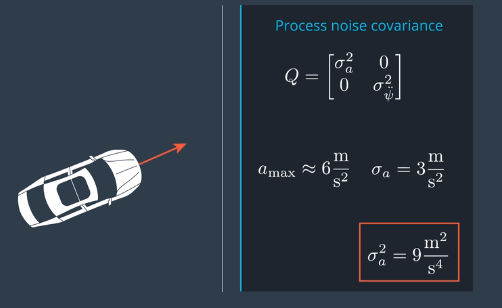
对于CTRV模型,两个参数定义了过程噪声:
- $\large \sigma^2_a$ 表示纵向加速度噪声(也被称为线性加速度)
- $\large \sigma^2_{\ddot\psi}$ 表示偏航加速度噪声(也称为角加速度)
在实际开发项目中,这两个值都需要调整。为了得到有效的解决方案,必须测试不同的值。在城市环境中考虑汽车的加速度情况,预期城市环境中的汽车加速或刹车的加速度通常不会超过 6 米每平方秒,选择预期最大加速度的一半作为过程噪音,通常可以使用 $\large \sigma^2_a = 9 \frac{m^2}{s^4}$作为跟踪车辆的起点。如果跟踪自行车以及行人等,9这个数字有点过于大,需要调整合适的参数。加速度噪声参数 $\large \sigma^2_a$ 的单位是 $\Large\frac{m^2}{s^4}$,取平方根,可以得到 $\large \sigma_a$ 的单位是 $\large \frac{m}{s^2}$,加速度噪声参数的平方根具有与加速度相同的单位。
参数$\large\sigma_a$是线性加速度的标准偏差。线性加速度被建模为具有均值为零和标准偏差$\large\sigma_a$的高斯分布。在高斯分布中,大约95%的值在$2\large\sigma_a$范围内,所以如果选择 $\large \sigma^2_a = 9 \frac{m^2}{s^4}$,你希望 95% 时间内加速度介于 $\large (-6 \frac{m}{s^2} , \large +6 \frac{m}{s^2})$。
让我们考虑偏航加速度噪声参数可能是哪些值。想象一下自行车以恒定的偏航率(角速度) $\Large \frac{\pi}{8} \frac{rad}{s}$在圆圈中行驶,这意味着自行车将在16秒内完成一整圈。 $\Large\frac{\pi}{8} \frac{rad}{s} \cdot 16 s = 2\pi$ 。意味着平均来说自行车的骑行半径为16米是合理值。自行车的切向速度为每秒6.28米, $\Large\frac{\pi}{8} \frac{rad}{s} \cdot 16 \text{ meters} = 6.28 \text{ meters per second}$。
如果角加速度现在是$\large-2\pi\frac{rad}{s^2}$而不是零?在一秒钟内,角速度将从 $\Large \frac{\pi}{8} \frac{rad}{s}$ 到 $\Large -\frac{15\pi}{8} \frac{rad}{s}$ 。自行车在16秒内完成了一个完整的循环。但是在如此高的角加速度下,自行车突然以相反的方向绕圈,只需要1.1秒就可以完成。对于自行车来说,设置 $\large \sigma_{\ddot\psi} = 2\pi \frac{rad}{s^2}$ 似乎太高了。
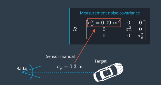
测量噪声参数表示传感器测量的不确定性。通常,制造商将在传感器手册中提供这些值,不需要调整这些参数。
一致性检查噪音参数设置是否正确
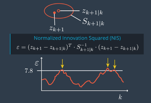
| 在每个时间循环里,计算每次预测的测量预测值 zk+1 | k以及协方差矩阵 S,我们收到该时间步的实际测量值 zk+1,实际测量值在误差椭圆内部,如果不在椭圆内部则可能噪音参数设置不正确。 |
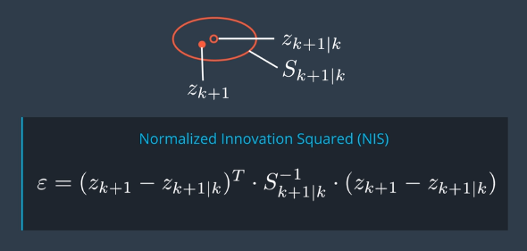
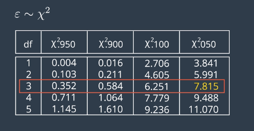
有种重要的一致性检查方法 NIS,NIS方法计算预测测量值和实际测量值之间的差,并对协方差矩阵 S 进行归一化。NIS 的值分布符合卡方分布。例如3个自由度的卡方分布,在所有情况下有 5% 的概率NIS 会超过 7.815,对每个时间步 k 计算并画出 NIS 值的表示图,以7.8为标线衡量,95%的值在标线以下则是正常的。
4.7 初始化卡尔曼滤波器
如前所述,过程噪声参数对卡尔曼滤波器有重要影响,作为开发项目的一部分,需要调整纵向和偏航加速度噪声参数。
状态变量的初始值也会影响卡尔曼滤波器的性能。状态向量X和状态协方差矩阵P需要初始化,UKF才能正常工作。
初始化状态向量 x
状态向量x包含 $x = [p_x, p_y, v, \psi, \dot{\psi}]$
在收到第一个传感器测量值之前,不知道自行车在哪里。第一次传感器测量到达,可以初始化$p_x$和$p_y$。
对于状态向量x中的其他变量,可以尝试不同的初始化值,以查看什么效果最好。
请注意,尽管雷达包含速度信息,但雷达速度和CTRV速度并不相同。从自动驾驶车辆的角度测量雷达速度。如果你画了一条从车辆到自行车的直线,雷达会测量这条直线上的速度。
在CTRV模型中,速度是从物体的角度来看的,在这种情况下,物体就是自行车;CTRV速度与自行车行驶的圆周相切。因此,不能直接使用雷达速度测量来初始化状态向量。
初始化状态协方差矩阵P
要初始化状态协方差矩阵P,一个选项是从单位矩阵开始。对于CTRV模型,P是一个5x5矩阵。单位矩阵将是:
\[P_{\text initial} = \begin{bmatrix} 1 \qquad 0 \qquad 0 \qquad 0 \qquad 0 \\ 0 \qquad 1 \qquad 0 \qquad 0 \qquad 0 \\ 0 \qquad 0 \qquad 1 \qquad 0 \qquad 0 \\ 0 \qquad 0 \qquad 0 \qquad 1 \qquad 0 \\ 0 \qquad 0 \qquad 0 \qquad 0 \qquad 1 \end{bmatrix}\]回想一下状态协方差矩阵表示的内容:以第一行第二列中的值为例。(1,2)处的值将是协方差 $\large \sigma_{px, py}$ 测量两个变量之间的线性关系。
对角线值表示x状态向量中每个变量的方差: $\large [\sigma^2{p_x}, \sigma^2{p_y}, \sigma^2{v}, \sigma^2{\psi}, \sigma^2_{\dot{\psi}}]$
为什么单位矩阵是一个好的起点?由于非对角值表示变量之间的协方差,因此P矩阵是对称的。单位矩阵也是对称的。对称来自两个变量之间的协方差是相同的,无论您查看$(x,y)$或$(y,x)$时,$\large \sigma_{px, py} = \sigma_{py, px}$。如果在UKF代码中打印出P矩阵,您将看到P即使在矩阵更新后仍保持对称。如果您的解决方案有效,您还将看到P开始相对快速地收敛到较小的值。
可以尝试将对角线值设置为真实状态和初始化的x状态向量之间的期望差值,而不是将每个对角线值设置为1。我们假设激光雷达x和y测量的标准偏差为0.15。如果以激光雷达测量值初始化 $p_x$ ,$p_x$中的初始方差或不确定性可能小于1。使用不同的初始化值进行实验,才能找到有效的解决方案。
5. 总结
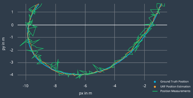
这里显示的是一辆自行车首先直线行驶然后沿圆形转弯。自行车的路径用蓝色表示,绿线是我们从激光雷达和雷达收到的所有测量值序列,这些测量值充满噪音。橙色的点是UKF 的融合了激光和雷达测量值的估算预测值。 CTRV 模型能很好地追踪拐弯,并且提供平滑的位置估算。可以调整过程噪音值让估算更加平滑,或者强迫噪音更快地跟上测量值。改变过程噪音值时,一定要检查滤波器的一致性。
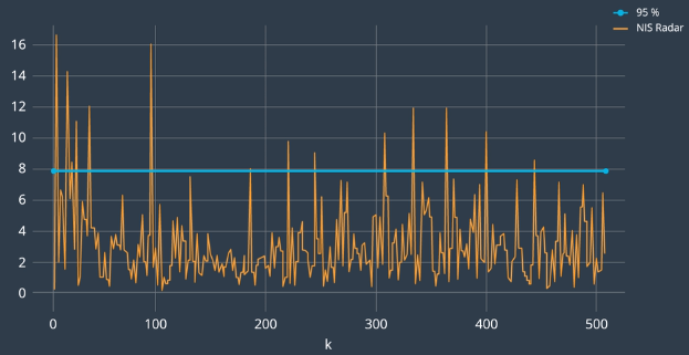
雷达测量值的一致性检查(NIS)如下图所示。和预期的一样,少量的 NIS 值超过了 95% 线(卡方值7.8)。
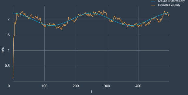
UKF 不管有没有雷达测速都能估算自行车的速度,当然如果有雷达测速,速度估算的收敛速度更快。
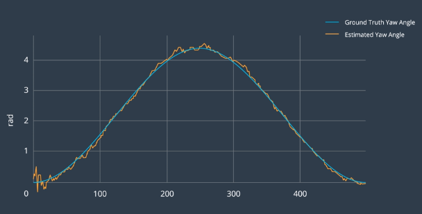
UKF在传感器无法直接观察方向的情况下,仍然能精确估计自行车的行驶方向。
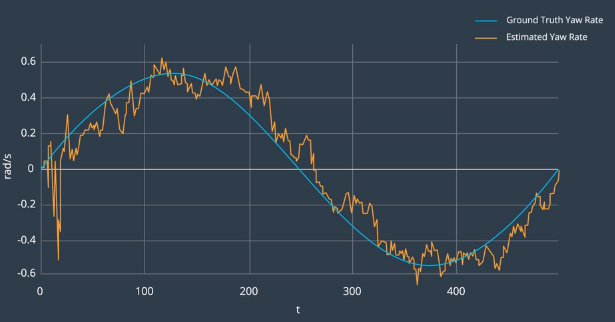
UKF甚至能直接估计出基本有用的自行车角速度。对于无人驾驶车,其他车辆的角速度很重要,角速度是车辆变道、转弯等危险行为最终的预测指标。
为什么卡尔曼滤波器对无人驾驶车而言是如此重要?
UKF 作为无人驾驶的传感器融合工具有三个最重要的功能。
第一,在 UKF 中,你可以输入噪音测量数据并获得周围动态对象的位置和速度的平滑估算,不会引发延时。
第二,即便使用的传感器无法直接观察,还是可以获得其他车辆的方向和角速度的估算。
第三,除此以外,UKF 还能给出结果的准确度。因为它能提供每个时间步状态估计的协方差矩阵。如果 UKF 已经执行了一致性检查,你就能知道协方差矩阵是贴近现实的。估算结果的不确定性对无人驾驶车非常重要,因为 如果在某个时刻前方车辆的位置非常不确定,最好多拉开点车距。
传感器融合是如何融入整个无人驾驶车技术栈的?
首先,传感器记录数据。
接下来,是预处理步骤,如使用聚类算法或更复杂的方案来检测对象假设。
最后,我们可以把这些假设作为对象级别融合的输入。
在传感器融合模块中,我们把所有数据整合到了一起,这并不是唯一的实现流程。每个处理步骤中都可以应用传感器融合。
保证了对周围世界的一致表述后,我们就可以把结果传递给无人驾驶车系统的下游环节,不同团队可以使用这些数据来定位车辆、控制车辆以及规划车辆路径。