传感器融合实时多目标物体对象追踪

1. 多目标追踪概述

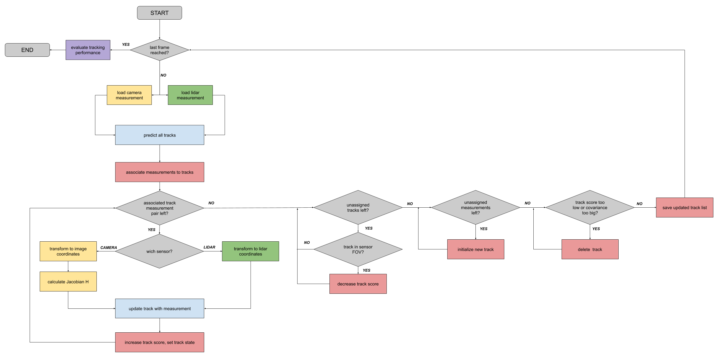
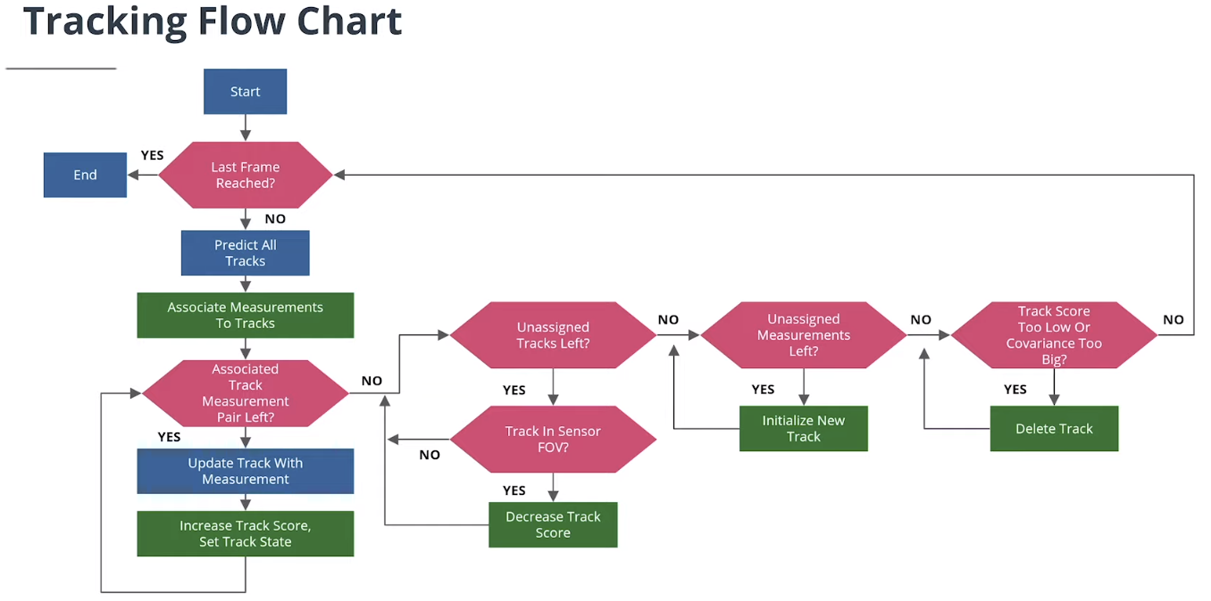
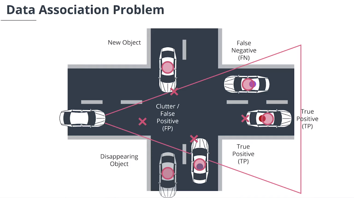
除单目标跟踪外，多目标跟踪系统还必须完成以下任务：

• 数据关联：
• • 将测量值与轨迹关联

• 追踪管理：

• • 初始化新跟踪对象
• • 删除旧跟踪对象
• • 给跟踪对象赋值置信度

2. 初始化追踪

2.1 状态初始化

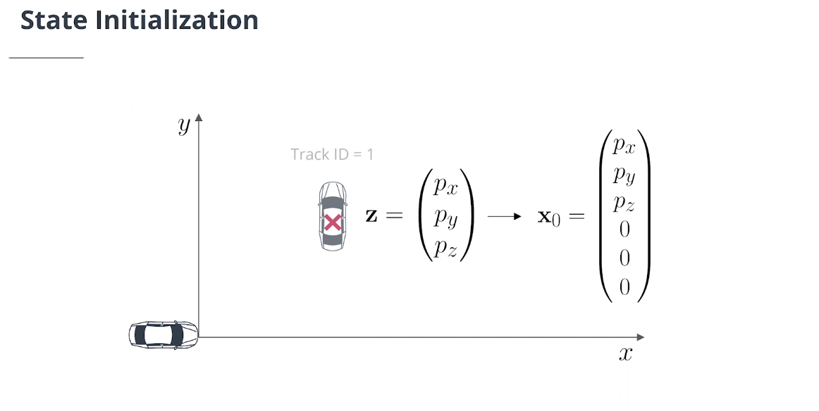
一个未分配的激光雷达测量$\mathbf z =（z_1，z_2，z_3）^ T$首先必须从传感器坐标转换为车辆坐标：

\[\begin{pmatrix} p_x\\ p_y\\p_z\\1 \end{pmatrix} = \left(\begin{array}{c|c} \begin{matrix} r_{11} & r_{12}& r_{13} \\ r_{21} & r_{22}& r_{23}\\ r_{31} & r_{32}& r_{33} \end{matrix} & \begin{matrix} t_1 \\ t_2\\ t_3 \end{matrix}\\ \overline{\begin{matrix} 0 &0&0 \end{matrix}} & \overline{\begin{matrix} 1 \end{matrix}} \end{array}\right) \cdot \begin{pmatrix} z_1\\ z_2\\z_3\\1 \end{pmatrix} = \left(\begin{array}{c|c} {\mathbf M_{\text{rot}}} & {\text t}\\ \overline{\begin{matrix} 0 &0&0 \end{matrix}} & \overline{\begin{matrix} 1 \end{matrix}} \end{array}\right) \cdot \begin{pmatrix} z_1\\ z_2\\z_3\\1 \end{pmatrix}\]

然后我们可以按如下方式初始化新追踪的状态：

\[\mathbf x_0 = \begin{pmatrix} p_x\\ p_y\\ p_z\\0\\0\\0 \end{pmatrix}\]

2.2 协方差初始化

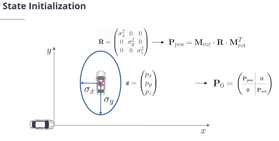
3x3的位置估计误差协方差矩阵$\mathbf p _ {\text {pos}}$可以通过从传感器坐标旋转到车辆坐标的测量协方差$\textbf R$初始化：

\[\mathbf P_{\text{pos}}= \mathbf M_{\text{rot}}\cdot \mathbf R \cdot \mathbf M_{\text{rot}}^T\]

3x3的速度估计误差协方差矩阵 $\mathbf P_{\text{vel}}$ 可以使用包含较大对角值的对角矩阵初始化，因为我们无法测量速度，因此具有巨大的初始速度不确定性。

可将总体估计误差协方差初始化为：

\[\mathbf P_0 = \left(\begin{array}{c|c} \underline{\mathbf P_{\text{pos}}} & {0}\\ {0} & \overline{\mathbf P_{\text{vel}}} \end{array}\right)\]

2.3 协方差旋转变换的推导

测量协方差$\text R$通过期望$E$定义：

\[\mathbf R = cov(\mathbf z) = E\left[(\mathbf z - E(\mathbf z))(\mathbf z - E(\mathbf z))^T\right]\]

记住测量方程：

\[\mathbf z = h(\mathbf x)+\omega\]

其中$ \omega \sim \mathcal{N}\left(0, \mathbf R\right)$是均值为0，协方差为$\text R$的测量噪声。由于ω均值为零，$\mathbf z$的期望仅为$h（\mathbf x）$：

\[E(\mathbf z) = E(h(\mathbf x)+\omega) = h(\mathbf x)\]

则有：

\[\mathbf R = E\left[(\mathbf z - E(\mathbf z))(\mathbf z - E(\mathbf z))^T\right]\] \[= E\left[(\mathbf h(\mathbf x)+\omega - E(h(\mathbf x)+\omega))(...)^T\right]\] \[= E\left[(\mathbf h(\mathbf x)+\omega - h(\mathbf x))(...)^T\right]\] \[= E\left[\omega \omega^T\right]\]

现在我们要将测量值从传感器旋转到车辆坐标，因此我们得到（注意$（\mathbf A\mathbf B）^T=\mathbf B^T\mathbf A^T$

\[\mathbf P_{\text{pos}} = E\left[\mathbf M_{\text{rot}}\omega \cdot(\mathbf M_{\text{rot}} \omega)^T\right]\] \[= E\left[\mathbf M_{\text{rot}}\omega \omega^T\mathbf M_{\text{rot}} ^T\right]\] \[= \mathbf M_{\text{rot}}E\left[\omega \omega^T\right]\mathbf M_{\text{rot}} ^T\] \[=\mathbf M_{\text{rot}}\cdot \mathbf R \cdot \mathbf M_{\text{rot}}^T\]

类似的推理同样可以应用于卡尔曼滤波方程的其他表达式。例如：

\[\mathbf P^- = \mathbf F\mathbf P^+\mathbf F^T+\mathbf Q\] \[\mathbf S = \mathbf H\mathbf P^+\mathbf H^T+\mathbf R\]

2.4 Python代码实现追踪初始化

import numpy as np
import matplotlib
matplotlib.use('wxagg') # change backend so that figure maximizing works on Mac as well  
import matplotlib.pyplot as plt
import matplotlib.ticker as ticker

class Track:
    '''Track class with state, covariance, id'''
    def __init__(self, meas, id):
        print('creating track no.', id)
        self.id = id

        # transform measurement to vehicle coordinates
        pos_sens = np.ones((4, 1)) # homogeneous coordinates
        pos_sens[0:3] = meas.z[0:3] 
        pos_veh = meas.sens_to_veh*pos_sens

        # save initial state from measurement
        self.x = np.zeros((6,1))
        self.x[0:3] = pos_veh[0:3]

        # set up position estimation error covariance
        M_rot = meas.sens_to_veh[0:3, 0:3]
        P_pos = M_rot * meas.R * np.transpose(M_rot)

        # set up velocity estimation error covariance
        sigma_p44 = 50 # initial setting for estimation error covariance P entry for vx
        sigma_p55 = 50 # initial setting for estimation error covariance P entry for vy
        sigma_p66 = 5 # initial setting for estimation error covariance P entry for vz
        P_vel = np.matrix([[sigma_p44**2, 0, 0],
                        [0, sigma_p55**2, 0],
                        [0, 0, sigma_p66**2]])

        # overall covariance initialization
        self.P = np.zeros((6, 6))
        self.P[0:3, 0:3] = P_pos
        self.P[3:6, 3:6] = P_vel


###################  

class Measurement:
    '''Lidar measurement class including measurement z, covariance R, coordinate transform matrix'''
    def __init__(self, gt, phi, t):
        # compute rotation around z axis
        M_rot = np.matrix([[np.cos(phi), -np.sin(phi), 0], 
                    [np.sin(phi), np.cos(phi), 0],
                    [0, 0, 1]])

        # coordiante transformation matrix from sensor to vehicle coordinates
        self.sens_to_veh = np.matrix(np.identity(4))            
        self.sens_to_veh[0:3, 0:3] = M_rot
        self.sens_to_veh[0:3, 3] = t
        print('Coordinate transformation matrix:', self.sens_to_veh)

        # transform ground truth from vehicle to sensor coordinates
        gt_veh = np.ones((4, 1)) # homogeneous coordinates
        gt_veh[0:3] = gt[0:3] 
        gt_sens = np.linalg.inv(self.sens_to_veh) * gt_veh

        # create measurement object
        sigma_lidar_x = 0.01 # standard deviation for noisy measurement generation
        sigma_lidar_y = 0.01
        sigma_lidar_z = 0.001
        self.z = np.zeros((3,1)) # measurement vector
        self.z[0] = float(gt_sens[0,0]) + np.random.normal(0, sigma_lidar_x)
        self.z[1] = float(gt_sens[1,0]) + np.random.normal(0, sigma_lidar_y)
        self.z[2] = float(gt_sens[2,0]) + np.random.normal(0, sigma_lidar_z)
        self.R = np.matrix([[sigma_lidar_x**2, 0, 0], # measurement noise covariance matrix
                            [0, sigma_lidar_y**2, 0], 
                            [0, 0, sigma_lidar_z**2]])

def visualize(track, meas):
    fig, (ax1, ax2, ax3) = plt.subplots(1,3)
    ax1.scatter(-meas.z[1], meas.z[0], marker='o', color='blue', label='measurement')
    ax2.scatter(-track.x[1], track.x[0], color='red', s=80, marker='x', label='initialized track')

    # transform measurement to vehicle coordinates for visualization
    z_sens = np.ones((4, 1)) # homogeneous coordinates
    z_sens[0:3] = meas.z[0:3] 
    z_veh = meas.sens_to_veh * z_sens
    ax3.scatter(-float(z_veh[1]), float(z_veh[0]), marker='o', color='blue', label='measurement')
    ax3.scatter(-track.x[1], track.x[0], color='red', s=80, marker='x', label='initialized track')

    # maximize window     
    mng = plt.get_current_fig_manager()
    mng.frame.Maximize(True)

    # legend and axes
    for ax in (ax1, ax2, ax3):
        ax.legend(loc='center left', shadow=True, fontsize='large', bbox_to_anchor=(0.5, 0.1))
        ax.set_xlabel('y [m]')
        ax.set_ylabel('x [m]')
        ax.set_xlim(-2,2)
        ax.set_ylim(0,2)
        # correct x ticks (positive to the left)
        ticks_x = ticker.FuncFormatter(lambda x, pos: '{0:g}'.format(-x) if x!=0 else '{0:g}'.format(x))
        ax.xaxis.set_major_formatter(ticks_x)

    # titles
    ax1.title.set_text('Sensor Coordinates')
    ax2.title.set_text('Vehicle Coordinates')
    ax3.title.set_text('Vehicle Coordinates\n (track and measurement should align)')

    plt.show()


###################  
# ground truth         
gt = np.matrix([[1.7],
                [1],
                [0]])

# sensor translation and rotation angle
t = np.matrix([[2],
                [0.5],
                [0]])
phi = np.radians(45)

# generate measurement
meas = Measurement(gt, phi, t)

# initialize track from this measurement
track = Track(meas, 1)

# visualization
visualize(track, meas)

3. 追踪状态管理

3.1 追踪分数评估

我们可以通过设置来定义一个简单的追踪分数：

\[\text{score} = \frac{\#\text{detections in last $n$ frames}}{n}\]

有许多其他的可能性来定义一个跟踪分数，信心或存在的概率。

基于追踪分数，可以定义追踪状态，例如“已初始化”、“暂定”或“已确认”。

示例跟踪删除条件

下面是一个启发式轨迹删除标准的示例：

• 确认追踪：

如果分数<0.6，则删除。这只适用于已确认的追踪，因此之前的分数必须高于0.8，然后降至0.6以下。

如果$\mathbf P_{11}<3^2$或$\mathbf P_{22}<3^2$则删除。这意味着我们的目标可能在半径为3米圆内的任何地方，位置不确定性增加了很多，因此追踪应该被删除。

• 暂定或初始化追踪：

如果分数<0.17，则删除。请注意，此阈值远低于已确认追踪的阈值，我们不希望在新追踪稳定之前立即删除它们。

如果$\mathbf P_{11}<3^2$，或$\mathbf P_{22}<3^2$则删除。

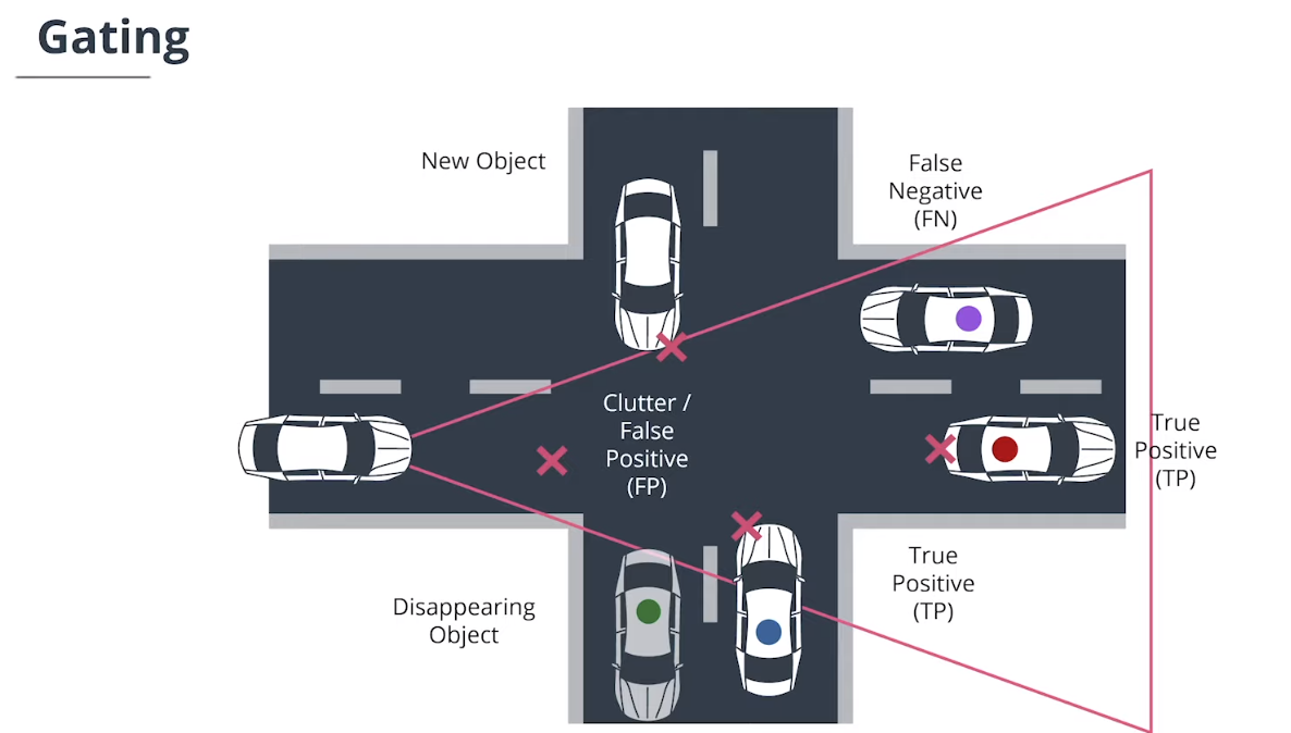
3.2 可见度

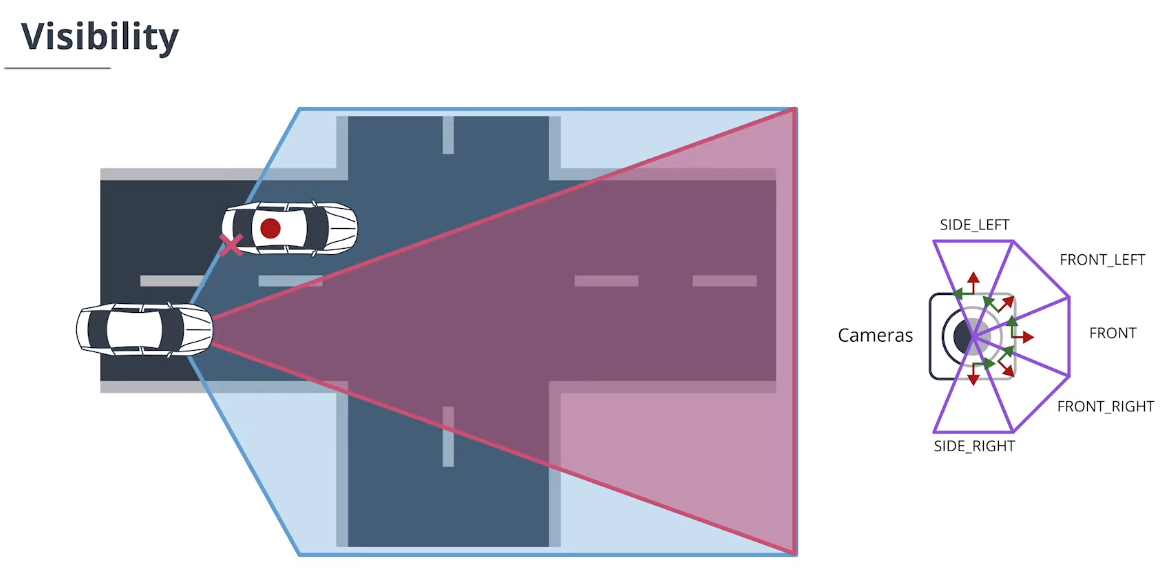
在传感器融合系统中，每个传感器通常具有不同的视野。我们需要一个检测概率或可见性推理来避免追踪分数振荡。

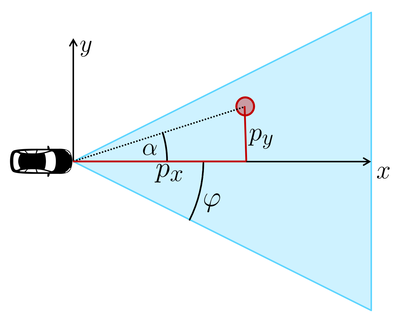
看看这张图片。我们想检查红色物体的可见性，它的坐标$p_x，p_y$已转换为此图像中的传感器坐标。我们必须计算红色目标相对于车辆的角度$α$。如果α的绝对值小于相机的开放角度$φ$，我们可以看到物体，否则我们看不到。那么我们如何计算α？

可以用三角函数计算$α$。我们已经知道对边$p_y$和邻边$p_x$，我们假设$p_x$>0，因此可以使用正切函数：

\[\tan(\alpha) = \frac{p_y}{p_x}\]

通过使用反正切函数即可求得所需的角度$\alpha$：

\[\alpha = \arctan\left(\frac{p_y}{p_x}\right)\]

3.3 Python实现相机追踪可视角度推理

# imports
import numpy as np
import matplotlib
#matplotlib.use('wxagg') # change backend so that figure maximizing works on Mac as well   
import matplotlib.pyplot as plt
import matplotlib.ticker as ticker

class Camera:
    '''Camera sensor class including field of view and coordinate transformation'''
    def __init__(self, phi, t):
        self.fov = [-np.pi/4, np.pi/4] # sensor field of view / opening angle

        # compute rotation around z axis
        M_rot = np.matrix([[np.cos(phi), -np.sin(phi), 0],
                    [np.sin(phi), np.cos(phi), 0],
                    [0, 0, 1]])
        print(M_rot)

        # coordiante transformation matrix from sensor to vehicle coordinates
        self.sens_to_veh = np.matrix(np.identity(4))            
        self.sens_to_veh[0:3, 0:3] = M_rot
        self.sens_to_veh[0:3, 3] = t
        self.veh_to_sens = np.linalg.inv(self.sens_to_veh) # transformation vehicle to sensor coordinates

    def in_fov(self, x):
        # check if an object x can be seen by this sensor
        pos_veh = np.ones((4, 1)) # homogeneous coordinates
        pos_veh[0:3] = x[0:3] 
        pos_sens = self.veh_to_sens*pos_veh # transform from vehicle to sensor coordinates
        visible = False
        # make sure to not divide by zero - we can exclude the whole negative x-range here
        if pos_sens[0] > 0: 
            alpha = np.arctan(pos_sens[1]/pos_sens[0]) # calc angle between object and x-axis
            # no normalization needed because returned alpha always lies between [-pi/2, pi/2]
            if alpha > self.fov[0] and alpha < self.fov[1]:
                visible = True

        return visible

#################
def run():
    '''generate random points and check visibility'''
    # camera with translation and rotation angle
    t = np.matrix([[2],
                    [0],
                    [0]])
    phi = np.radians(45)
    cam = Camera(phi, t)

    # initialize visualization
    fig, ax = plt.subplots()

    for i in range(50):
        # define track position and velocity
        x = np.matrix([[np.random.uniform(-5,5)],
                    [np.random.uniform(-5,5)],
                    [0],
                    [0],
                    [0],
                    [0]])

        # check if x is visible by camera
        result = cam.in_fov(x)

        # plot results
        pos_veh = np.ones((4, 1)) # homogeneous coordinates
        pos_veh[0:3] = x[0:3] 
        pos_sens = cam.veh_to_sens*pos_veh # transform from vehicle to sensor coordinates
        if result == True:
            col = 'green'
            ax.scatter(float(-pos_sens[1]), float(pos_sens[0]), marker='o', color=col, label='visible track')
        else:
            col = 'red'
            ax.scatter(float(-pos_sens[1]), float(pos_sens[0]), marker='o', color=col, label='invisible track')
        ax.text(float(-pos_sens[1]), float(pos_sens[0]), str(result))

    # plot FOV    
    ax.plot([0, -5], [0, 5], color='blue', label='field of view') 
    ax.plot([0, 5], [0, 5], color='blue')

    # maximize window     
    mng = plt.get_current_fig_manager()
    #mng.frame.Maximize(True)

    # remove repeated labels
    handles, labels = ax.get_legend_handles_labels()
    handle_list, label_list = [], []
    for handle, label in zip(handles, labels):
        if label not in label_list:
            handle_list.append(handle)
            label_list.append(label)
    ax.legend(handle_list, label_list, loc='center left', shadow=True, fontsize='large', bbox_to_anchor=(0.9, 0.1))

    # axis
    ax.set_xlabel('y [m]')
    ax.set_ylabel('x [m]')
    ax.set_xlim(-5,5)
    ax.set_ylim(0,5)

    # correct x ticks (positive to the left)
    ticks_x = ticker.FuncFormatter(lambda x, pos: '{0:g}'.format(-x) if x!=0 else '{0:g}'.format(x))
    ax.xaxis.set_major_formatter(ticks_x)

    plt.show() 

####################
# call main loop
run()

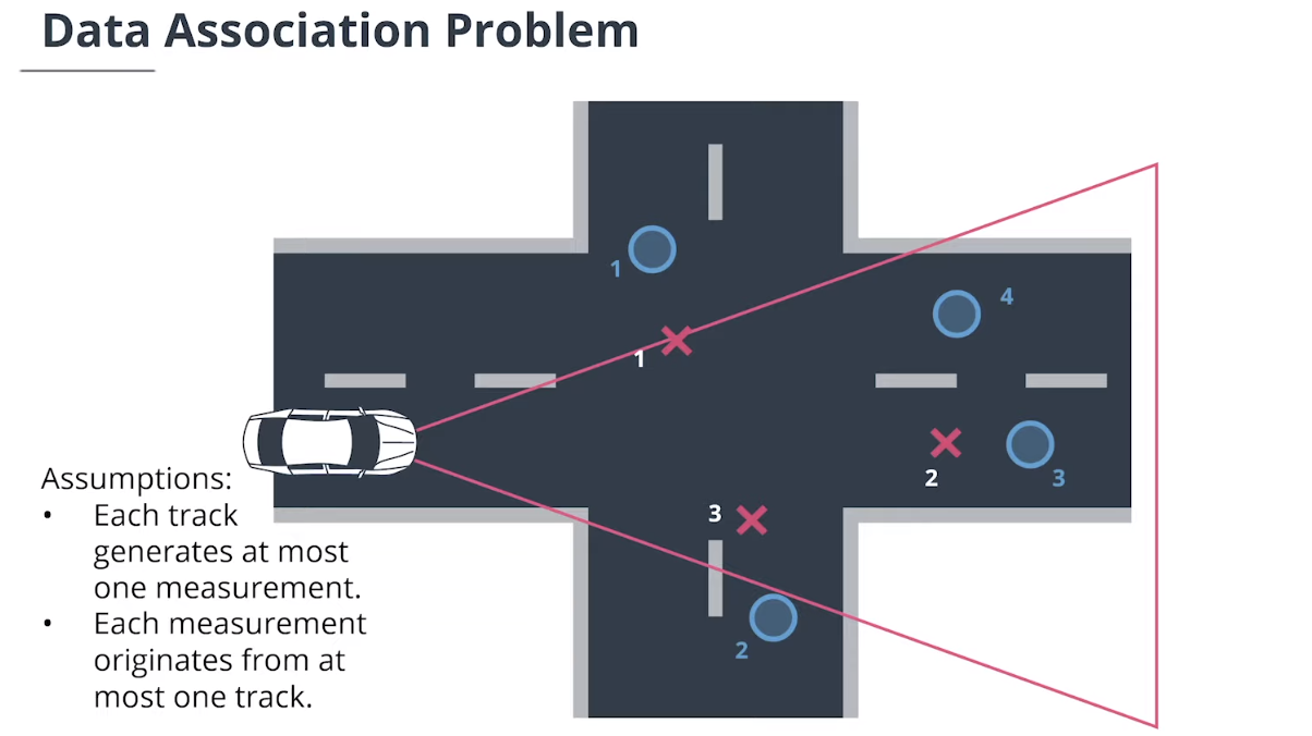
4. 数据关联

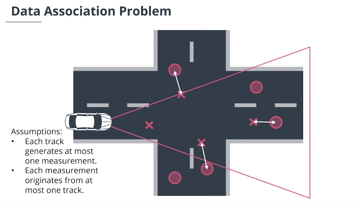
$\textbf{data association}$数据关联模块分配测量值给追踪，并决定哪个跟踪使用哪个测量值。

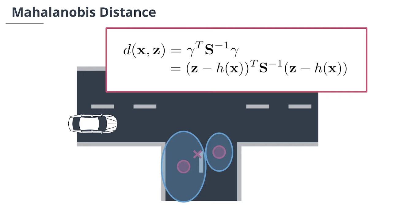
$\textbf{data association}$数据关联模块主要使用$\textbf{Mahalanobis distance}$马氏距离来做决定。

\[d(\mathbf x, \mathbf z)= \gamma^T\mathbf S^{-1}\gamma = (\mathbf z - h(\mathbf x))^T\mathbf S^{-1}(\mathbf z - h(\mathbf x))\]

4.1 数据关联方法概述

$\textbf{Simple Nearest Neighbor（SNN）}$简单最近邻数据关联计算追踪和测量值之间的所有马氏距离，然后迭代更新最近关联对。

SNN不是全局最优的，这可以使用$\textbf{Global Nearest Neighbor（GNN）}$全局最近邻数据关联来解决。

这两种数据关联方法都在不明确的情况下强制执行硬决策。更高级的$\textbf{Probabilistic Data Association（PDA）}$概率数据关联（PDA）技术可以避免这些困难的决策和由此产生的错误。此类有不同的变体（例如PDA、JPDA、JIPDA）。

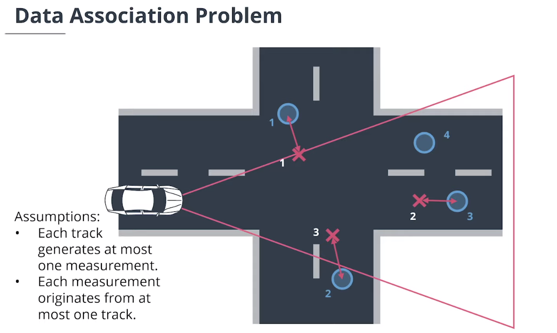
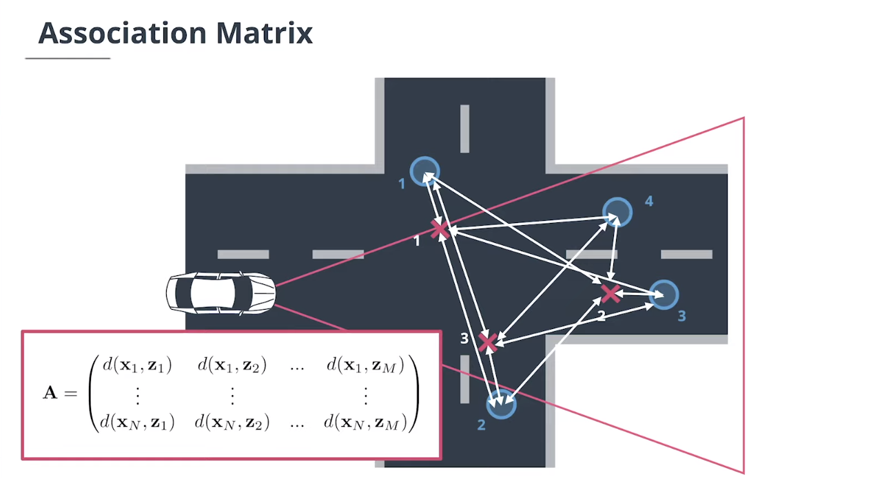
4.2 数据关联矩阵

假设我们有$N$个追踪目标轨迹和$M$个测量值。

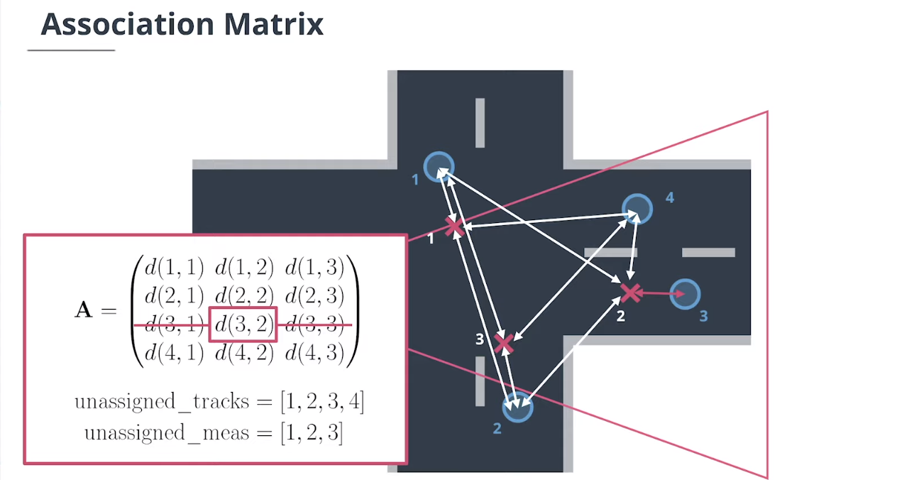
$\textbf{association matrix}$关联矩阵$\mathbf A$是一个$N×M$的矩阵，它包含每个追踪和每个测量之间的马氏距离：

\[\mathbf A = \begin{pmatrix} d(\mathbf x_1, \mathbf z_1) & d(\mathbf x_1, \mathbf z_2) &...&d(\mathbf x_1, \mathbf z_M)\\ \vdots &\vdots&&\vdots\\ d(\mathbf x_N, \mathbf z_1) & d(\mathbf x_N, \mathbf z_2) &...&d(\mathbf x_N, \mathbf z_M) \end{pmatrix}\]

我们还需要一个未指定追踪的列表和一个未指定测量的列表。

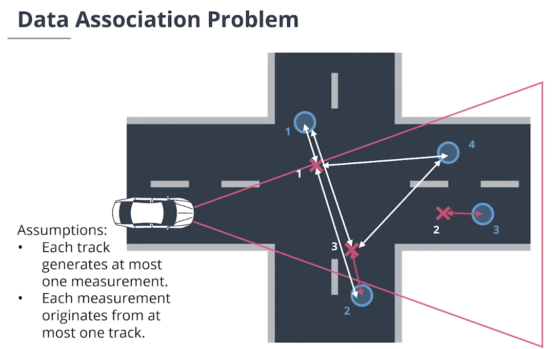
我们在$A$中查找最小的条目，以确定使用哪个度量更新哪个追踪，然后从$A$中删除该行和列，并从列表中删除追踪ID和度量ID。我们重复这个过程，直到$A$为空。

4.3 Python实现数据关联矩阵

import numpy as np
import matplotlib
matplotlib.use('wxagg') # change backend so that figure maximizing works on Mac as well   
import matplotlib.pyplot as plt
import matplotlib.ticker as ticker

class Association:
    '''Data association class with single nearest neighbor association and gating based on Mahalanobis distance'''
    def __init__(self):
        self.association_matrix = np.matrix([])

    def associate(self, track_list, meas_list):
        N = len(track_list) # N tracks
        M = len(meas_list) # M measurements

        # initialize association matrix
        self.association_matrix = np.inf*np.ones((N,M)) 

        # loop over all tracks and all measurements to set up association matrix
        for i in range(N): 
            track = track_list[i]
            for j in range(M):
                meas = meas_list[j]
                dist = self.MHD(track, meas)
                self.association_matrix[i,j] = dist

    def MHD(self, track, meas):
        # calc Mahalanobis distance
        H = np.matrix([[1, 0, 0, 0],
                       [0, 1, 0, 0]]) 
        gamma = meas.z - H*track.x
        S = H*track.P*H.transpose() + meas.R
        MHD = gamma.transpose()*np.linalg.inv(S)*gamma # Mahalanobis distance formula
        return MHD


################## 
class Track:
    '''Track class with state, covariance, id'''
    def __init__(self, id):
        # save id
        self.id = id

        # generate random state x
        self.x = np.matrix([[np.random.uniform(2,8)],
                        [np.random.uniform(-3,3)],
                        [0],
                        [0]])

        # set up estimation error covariance
        self.P = np.matrix([[2, 0, 0, 0],
                        [0, 3, 0, 0],
                        [0, 0, 1, 0],
                        [0, 0, 0, 1]])

class Measurement:
    '''Measurement class with easurement, covariance, id'''
    def __init__(self, id, x, y):
        # save id
        self.id = id

        # generate random measurement z
        self.z = np.matrix([[x + np.random.normal(0,2)],
                        [y + np.random.normal(0,2)]])

        # set up measurement covariance
        self.R = np.matrix([[2, 0],
                        [0, 2]])


#################
def run():
    '''generate tracks and measurements and call association'''
    # set up track_list and meas_list for association
    np.random.seed(5) # make random values predictable
    association = Association() # init data association
    track_list = []
    meas_list = []

    # initialize visualization
    fig, ax = plt.subplots()

    # generate and plot tracks and measurements
    for i in range(3):

        # tracks
        track = Track(i+1)
        track_list.append(track)
        ax.scatter(float(-track.x[1]), float(track.x[0]), marker='x', color='red', label='track')
        ax.text(float(-track.x[1]), float(track.x[0]), str(track.id), color='red')

        # measurements
        meas = Measurement(i+1, float(track.x[0]), float(track.x[1]))
        meas_list.append(meas)
        ax.scatter(float(-meas.z[1]), float(meas.z[0]), marker='o', color='green', label='measurement')
        ax.text(float(-meas.z[1]), float(meas.z[0]), str(meas.id), color='green')

    # calculate association matrix
    association.associate(track_list, meas_list)
    print('Association matrix:', association.association_matrix)

    # visualize distances
    for track in track_list:
        for meas in meas_list:
            dist = association.association_matrix[track.id-1, meas.id-1]
            if dist < np.inf: 
                ax.plot([float(-track.x[1]), float(-meas.z[1])], [float(track.x[0]), float(meas.z[0])], color='gray')
                str_dist = "{:.2f}".format(dist)
                ax.text(float((-track.x[1] - meas.z[1])/2), float((track.x[0] + meas.z[0])/2), str_dist)

    # maximize window     
    mng = plt.get_current_fig_manager()
    mng.frame.Maximize(True)

    # remove repeated labels
    handles, labels = ax.get_legend_handles_labels()
    handle_list, label_list = [], []
    for handle, label in zip(handles, labels):
        if label not in label_list:
            handle_list.append(handle)
            label_list.append(label)
    ax.legend(handle_list, label_list, loc='center left', shadow=True, fontsize='large', bbox_to_anchor=(0.9, 0.1))

    # axis
    ax.set_xlabel('y [m]')
    ax.set_ylabel('x [m]')
    ax.set_xlim(-5,5)
    ax.set_ylim(0,10)

    # correct x ticks (positive to the left)
    ticks_x = ticker.FuncFormatter(lambda x, pos: '{0:g}'.format(-x) if x!=0 else '{0:g}'.format(x))
    ax.xaxis.set_major_formatter(ticks_x)

    plt.show() 

####################
# call main loop
run()

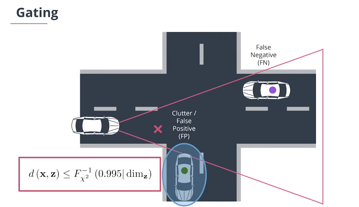
4.4 门控技术（Gating）

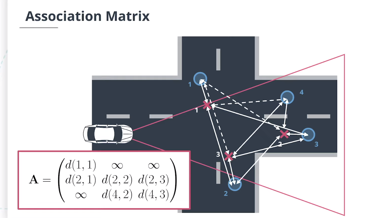
$Gating$门控技术通过删除不太可能的关联对来降低关联复杂性。

因为残差是高斯分布的，所以马氏距离遵循$\chi^2$分布。如果马氏距离小于通过逆累积$\chi^2$分布计算得出的阈值，则测量值位于追踪门内，阈值计算方式如下：

\[d\left(\mathbf x,\mathbf z\right)\leq F_{\chi^2}^{-1}\left(0.995|\dim_{\mathbf z}\right)\]

如果测量值位于追踪门控外，我们可以将其马氏距离设置为无穷大，例如：

\[\mathbf A = \begin{pmatrix} d(1, 1) & \infty &\infty \\ d(2, 1) & d(2, 2) &d(2, 3) \\ d(3, 1) & d(3, 2) &d(3, 3) \\ \infty& d(4, 2) &d(4, 3) \end{pmatrix}\]

计算逆累积$\chi^2$分布 $F_{\chi^2}^{-1}\left(p

df\right)$使用概率$p$和自由度$df$（等于此处测量空间的尺寸），可以使用scipy软件包：

  from scipy.stats.distributions import chi2

  chi2.ppf(p, df)

ppf代表百分点函数，它是累积密度函数的倒数。有关更多详细信息，请参阅相关的scipy文档。

要获取关联矩阵$A$中最小项的索引，可以使用numpy.argmin。通常，此函数返回展平数组的索引。为了避免这种情况，我们可以使用numpy.unravel_index，如下所示：

  np.unravel_index(np.argmin(A, axis=None), A.shape)

4.5 Python实现数据关联门控技术

import numpy as np
import matplotlib
matplotlib.use('wxagg') # change backend so that figure maximizing works on Mac as well   
import matplotlib.pyplot as plt
import matplotlib.ticker as ticker
from scipy.stats.distributions import chi2

class Association:
    '''Data association class with single nearest neighbor association and gating based on Mahalanobis distance'''
    def __init__(self):
        self.association_matrix = np.matrix([])
        self.unassigned_tracks = []
        self.unassigned_meas = []

    def associate(self, track_list, meas_list):
        N = len(track_list) # N tracks
        M = len(meas_list) # M measurements
        self.unassigned_tracks = list(range(N))
        self.unassigned_meas = list(range(M))

        # initialize association matrix
        self.association_matrix = np.inf*np.ones((N,M)) 

        # loop over all tracks and all measurements to set up association matrix
        for i in range(N): 
            track = track_list[i]
            for j in range(M):
                meas = meas_list[j]
                dist = self.MHD(track, meas)
                if self.gating(dist):
                    self.association_matrix[i,j] = dist

    def MHD(self, track, meas):
        # calc Mahalanobis distance
        H = np.matrix([[1, 0, 0, 0],
                       [0, 1, 0, 0]]) 
        gamma = meas.z - H*track.x
        S = H*track.P*H.transpose() + meas.R
        MHD = gamma.transpose()*np.linalg.inv(S)*gamma # Mahalanobis distance formula
        return MHD

    def gating(self, MHD): 
        # check if measurement lies inside gate
        limit = chi2.ppf(0.95, df=2)
        if MHD < limit:
            return True
        else:
            return False

    def get_closest_track_and_meas(self):
        # find closest track and measurement for next update
        A = self.association_matrix
        if np.min(A) == np.inf:
            return np.nan, np.nan

        # get indices of minimum entry
        ij_min = np.unravel_index(np.argmin(A, axis=None), A.shape) 
        ind_track = ij_min[0]
        ind_meas = ij_min[1]

        # delete row and column for next update
        A = np.delete(A, ind_track, 0) 
        A = np.delete(A, ind_meas, 1)
        self.association_matrix = A

        # update this track with this measurement
        update_track = self.unassigned_tracks[ind_track] 
        update_meas = self.unassigned_meas[ind_meas]

        # remove this track and measurement from list
        self.unassigned_tracks.remove(update_track) 
        self.unassigned_meas.remove(update_meas)

        return update_track, update_meas

################## 
class Track:
    '''Track class with state, covariance, id'''
    def __init__(self, id):
        # save id
        self.id = id

        # generate random state x
        self.x = np.matrix([[np.random.uniform(2,8)],
                        [np.random.uniform(-3,3)],
                        [0],
                        [0]])

        # set up estimation error covariance
        self.P = np.matrix([[2, 0, 0, 0],
                        [0, 3, 0, 0],
                        [0, 0, 1, 0],
                        [0, 0, 0, 1]])

class Measurement:
    '''Measurement class with easurement, covariance, id'''
    def __init__(self, id, x, y):
        # save id
        self.id = id

        # generate random measurement z
        self.z = np.matrix([[x + np.random.normal(0,2)],
                        [y + np.random.normal(0,2)]])

        # set up measurement covariance
        self.R = np.matrix([[2, 0],
                        [0, 2]])


#################
def run():
    '''generate tracks and measurements and call association'''
    # set up track_list and meas_list for association
    np.random.seed(5) # make random values predictable
    association = Association() # init data association
    track_list = []
    meas_list = []

    # initialize visualization
    fig, ax = plt.subplots()

    # generate and plot tracks and measurements
    for i in range(3):

        # tracks
        track = Track(i+1)
        track_list.append(track)
        ax.scatter(float(-track.x[1]), float(track.x[0]), marker='x', color='red', label='track')
        ax.text(float(-track.x[1]), float(track.x[0]), str(track.id), color='red')

        # measurements
        meas = Measurement(i+1, float(track.x[0]), float(track.x[1]))
        meas_list.append(meas)
        ax.scatter(float(-meas.z[1]), float(meas.z[0]), marker='o', color='green', label='measurement')
        ax.text(float(-meas.z[1]), float(meas.z[0]), str(meas.id), color='green')

    # calculate association matrix
    association.associate(track_list, meas_list)
    print('Association matrix:', association.association_matrix)
    print('unassigned_tracks list:', association.unassigned_tracks)
    print('unassigned_meas list:', association.unassigned_meas)     

    # visualize distances
    for track in track_list:
        for meas in meas_list:
            dist = association.association_matrix[track.id-1, meas.id-1]
            if dist < np.inf: 
                ax.plot([float(-track.x[1]), float(-meas.z[1])], [float(track.x[0]), float(meas.z[0])], color='gray')
                str_dist = "{:.2f}".format(dist)
                ax.text(float((-track.x[1] - meas.z[1])/2), float((track.x[0] + meas.z[0])/2), str_dist)

    # update associated tracks with measurements
    matrix_orig = association.association_matrix
    while association.association_matrix.shape[0]>0 and association.association_matrix.shape[1]>0:

        # search for next association between a track and a measurement
        ind_track, ind_meas = association.get_closest_track_and_meas()
        if np.isnan(ind_track):
            print('---no more associations---')
            break

        track = track_list[ind_track]
        meas = meas_list[ind_meas]
        dist = matrix_orig[ind_track, ind_meas]
        ax.plot([float(-track.x[1]), float(-meas.z[1])], [float(track.x[0]), float(meas.z[0])], color='blue', label='association')
        str_dist = "{:.2f}".format(dist)
        ax.text(float((-track.x[1] - meas.z[1])/2), float((track.x[0] + meas.z[0])/2), str_dist)
        print('found association between track', ind_track+1, 'and measurement', ind_meas+1, 'with MHD =', str_dist)
        print('New association matrix:', association.association_matrix)    
        print('New unassigned_tracks list:', association.unassigned_tracks)
        print('New unassigned_meas list:', association.unassigned_meas)        


    #################
    # visualization
    # maximize window     
    mng = plt.get_current_fig_manager()
    mng.frame.Maximize(True)

    # remove repeated labels
    handles, labels = ax.get_legend_handles_labels()
    handle_list, label_list = [], []
    for handle, label in zip(handles, labels):
        if label not in label_list:
            handle_list.append(handle)
            label_list.append(label)
    ax.legend(handle_list, label_list, loc='center left', shadow=True, fontsize='large', bbox_to_anchor=(0.9, 0.1))

    # axis
    ax.set_xlabel('y [m]')
    ax.set_ylabel('x [m]')
    ax.set_xlim(-5,5)
    ax.set_ylim(0,10)

    # correct x ticks (positive to the left)
    ticks_x = ticker.FuncFormatter(lambda x, pos: '{0:g}'.format(-x) if x!=0 else '{0:g}'.format(x))
    ax.xaxis.set_major_formatter(ticks_x)

    plt.show() 

####################
# call main loop
run()

5. 评估跟踪性能

为了评估跟踪性能，我们可以使用$\textbf{Root Mean Square Error（RMSE）}$均方根误差，它计算估计状态和基本真值状态之间的残差：

\[RMSE = \sqrt{\frac 1n\sum_{k=1}^n \left(x_k^{\text{est}}-x_k^{\text{true}}\right)^2}\]

回首页