扩展卡尔曼滤波器(EKF)2D物体对象追踪

1. 介绍

在本部分将介绍如何使用扩展卡尔曼滤波器融合激光雷达和相机测量,并在Python中实现2D Kalman过滤器以及非线性摄影机测量模型，以随时间跟踪对象。

2. 传感器融合概述

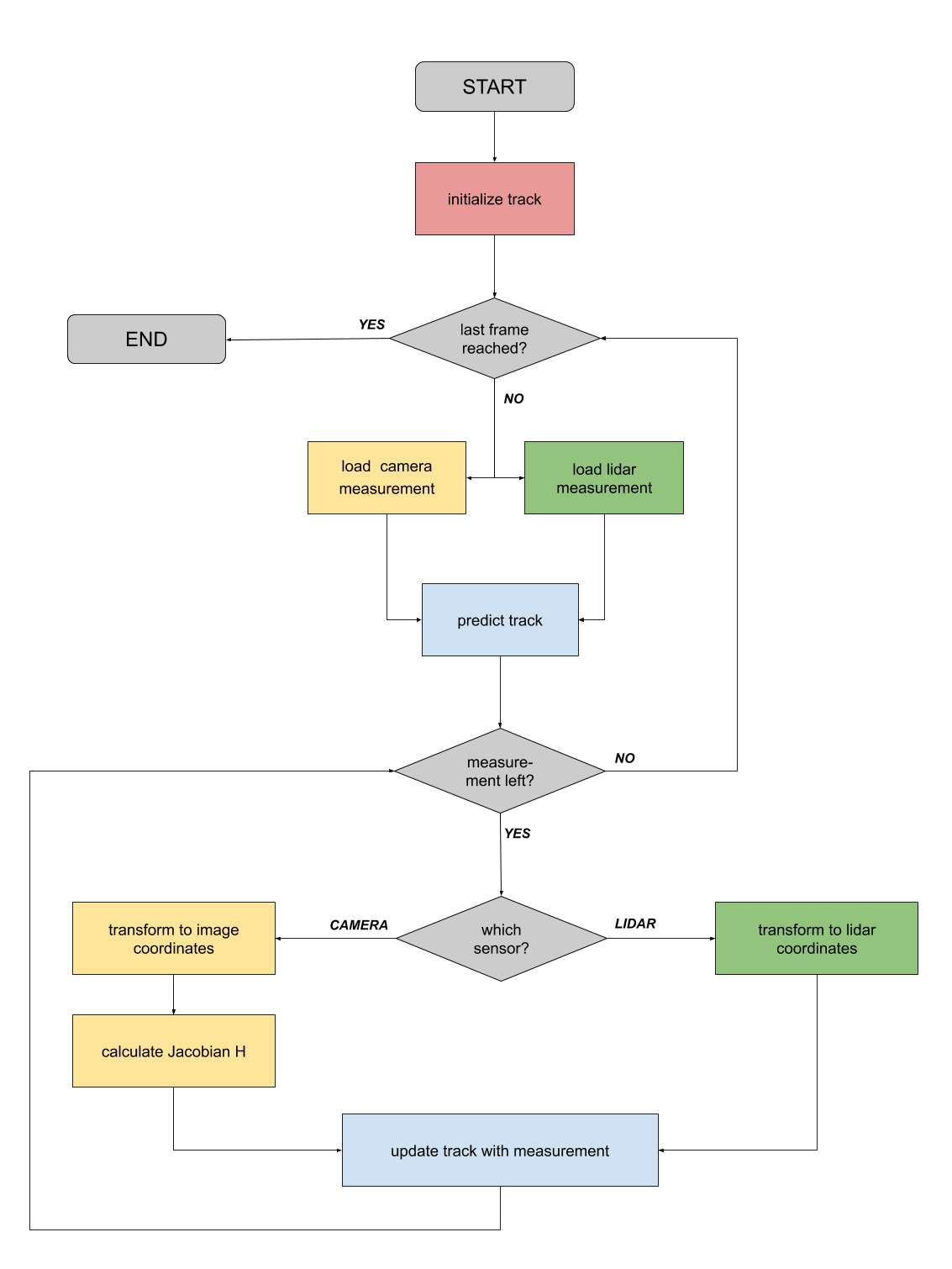
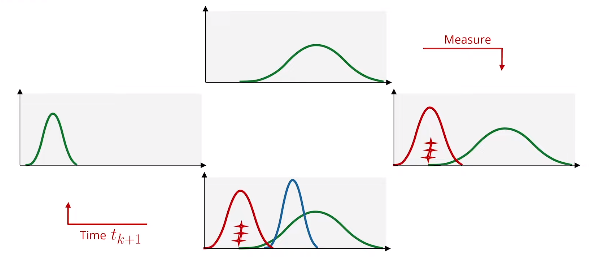
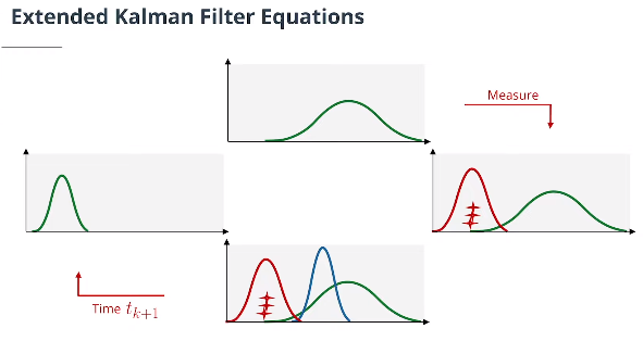
卡尔曼滤波算法将通过以下步骤随时间跟踪对象：

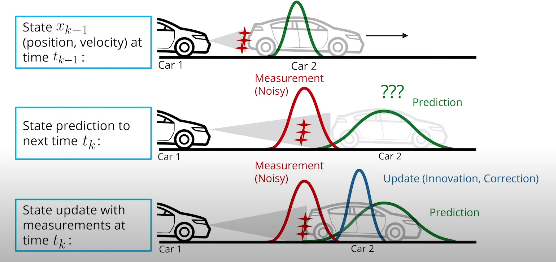
• 第一次测量:过滤器将接收物体相对于汽车位置的初始测量值,这些测量将来自摄像机或激光雷达传感器。

• 初始化状态和协方差矩阵:过滤器将基于第一次测量初始化对象的位置 $\begin{pmatrix} p_x \ p_y \end{pmatrix}$ 和速度 $\begin{pmatrix} v_x \ v_y \end{pmatrix}$ 。

• 汽车将在时间段$Δt$之后接收另一个传感器测量。

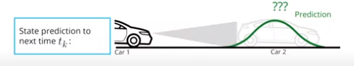
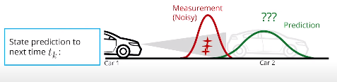
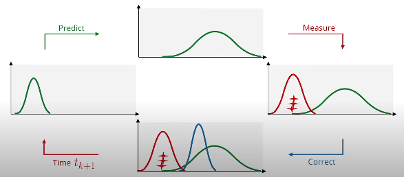
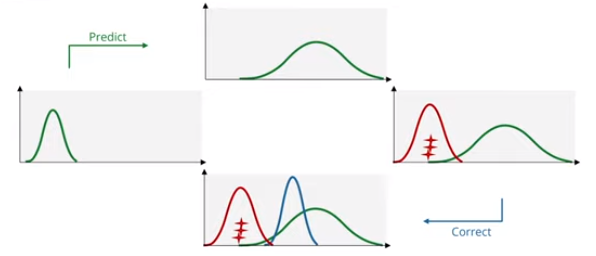
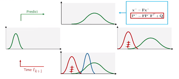
• 预测:算法将预测对象在时间$Δt$后的位置。

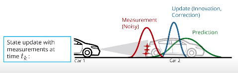
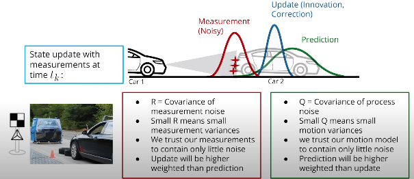
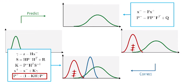
• 更新:过滤器将“预测”位置与传感器测量值进行比较,以给出更新的位置。根据每个值的不确定性，卡尔曼滤波器将对预测位置或测量位置施加更多权重。更新步骤通常也称纠正步骤。

• 汽车将在时间段$\ Δt$之后接收另一个传感器测量。然后算法进行另一个预测和更新步骤循环。

3. 估计问题概述

• 问题定义

• 变量定义

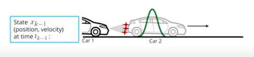
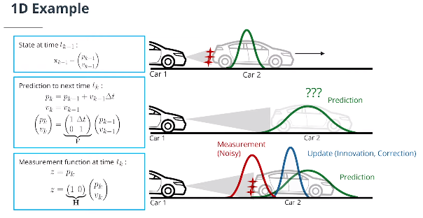
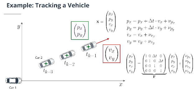
$\mathbf{ x}$是状态向量。它包含有关要跟踪的对象的位置和速度的信息：

\[\mathbf{ x} = \begin{pmatrix} p_x \\ p_y \\ v_x \\ v_y \end{pmatrix}\]

位置和速度由平均值为$\mathbf{x}$的高斯分布表示。$P$是估计误差协方差矩阵，其中包含有关对象位置和速度不确定性的信息。可以将其视为包含标准偏差。

$k$指时间步长索引，$x_k$是时间$t_k$时物体的位置和速度矢量。

$\ Δt$是两次连续测量之间的时间步长。

符号$\mathbf x_k^-$指预测步骤。在时间$t_k$，收到一个传感器测量值。在考虑传感器测量值以更新对对象位置和速度的信念之前，可以预测在$t_k$时对象的位置。可以基于时间$t_{k-1}$的位置和速度预测物体在$t_k$的位置。因此$\mathbf x_k^-$意味着已经预测了物体在$t_k$的位置，但尚未考虑新的传感器测量值。相应的预测协方差表示为$\mathbf P_k^-$。

$\mathbf x_k^+$意味着在预测了对象在时间$t_k$的位置后使用传感器测量值更新了对象的位置和速度。同样，更新后的协方差为$\mathbf P_k^+$。

4. 卡尔曼滤波器概述（1D直线运动）

4.1 状态转换函数和测量函数

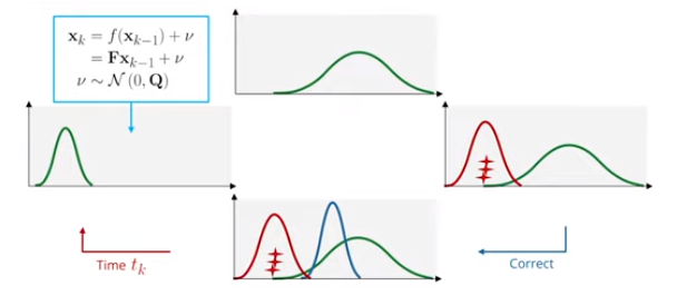
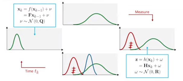
$f$是状态转换函数（在线性情况下，它是矩阵$\mathbf F$，也称为系统矩阵）。它告诉我们如何从一个时间戳到下一个时间戳：

\[x_k = f(x_{k-1})+\nu= \mathbf Fx_{k-1}+\nu\]

$\nu \sim \mathcal{N}\left(0, \mathbf Q\right)$ 是均值为0，协方差为 $\mathbf Q$ 的过程噪音

$h$是测量函数（在线性情况下，它是一个矩阵$\mathbf H$）。它告诉我们状态和测量是如何关联的：

\[z_k = h(x_k)+\omega= \mathbf Hx_k+\omega\]

$\omega \sim \mathcal{N}\left(0, \mathbf R\right)$ 是均值为0，协方差为$R$ 的测量噪音

$\mathbf z$是测量向量。

4.2 卡尔曼滤波方程综述

• 预测步骤：

\[\mathbf x^-=\mathbf F\mathbf x^+\] \[\mathbf P^-=\mathbf F\mathbf P^+\mathbf F^T+\mathbf Q\]

• 更新步骤：

\[\gamma = \mathbf z- \mathbf H\mathbf x\] \[\mathbf S = \mathbf H\mathbf P^- \mathbf H^T+\mathbf R\] \[\mathbf K = \mathbf P^- \mathbf H^T\mathbf S^{-1}\] \[\mathbf x^+ = \mathbf x^- +\mathbf K\gamma\] \[\mathbf P^+ = \left(\mathbf I - \mathbf K\mathbf H \right)\mathbf P^-\]

$\gamma = \mathbf z- \mathbf H\mathbf x$ 具有协方差 $\mathbf S = \mathbf H\mathbf P \mathbf H^T+\mathbf R$ 的残差

$\mathbf K = \mathbf P \mathbf H^T\mathbf S^{-1}$ 是卡尔曼增益参数Kalman gain，卡尔曼增益参数决定预测与测量的权重比例。

4.3 python实现卡尔曼滤波器

import numpy as np

class Filter:
    '''Kalman filter class'''
    def __init__(self):
        self.dim_state = 2 # process model dimension

    def F(self):
        # system matrix
        return np.matrix([[1, 1],
                        [0, 1]])

    def Q(self):
        # process noise covariance Q
        return np.matrix([[0, 0],
                        [0, 0]])

    def H(self):
        # measurement matrix H
        return np.matrix([[1, 0]])

    def predict(self, x, P):
        # predict state and estimation error covariance to next timestep
        F = self.F()
        x = F*x # state prediction
        P = F*P*F.transpose() + self.Q() # covariance prediction
        return x, P

    def update(self, x, P, z, R):
        # update state and covariance with associated measurement
        H = self.H() # measurement matrix
        gamma = z - H*x # residual
        S = H*P*H.transpose() + R # covariance of residual
        K = P*H.transpose()*np.linalg.inv(S) # Kalman gain
        x = x + K*gamma # state update
        I = np.identity(self.dim_state)
        P = (I - K*H) * P # covariance update
        return x, P     


def run_filter():
    ''' loop over data and call predict and update'''
    np.random.seed(10) # make random values predictable

    # init filter
    KF = Filter()

    # init track state and covariance
    x = np.matrix([[0],
                [0]])
    P = np.matrix([[5**2, 0],
                [0, 5**2]])  

    # loop over measurements and call predict and update
    for i in range(1,101):        
        print('------------------------------')
        print('processing measurement #' + str(i))

        # prediction
        x, P = KF.predict(x, P) # predict to next timestep
        print('x- =', x)
        print('P- =', P)

        # measurement generation
        sigma_z = 1 # measurement noise
        z = np.matrix([[i + np.random.normal(0, sigma_z)]]) # generate noisy measurement
        R = np.matrix([[sigma_z**2]]) # measurement covariance
        print('z =', z)

        # update
        x, P = KF.update(x, P, z, R) # update with measurement
        print('x+ =', x)
        print('P+ =', P)


# call main loop
run_filter()

5. 融合激光雷达与相机测量数据追踪对象（2D运动模式）

5.1 预测步骤

• 状态预测

对于二维运动,假设速度恒定，系统矩阵为：

\[\mathbf{F}(\Delta t) = \begin{pmatrix} 1 & 0 & \Delta t & 0 \\ 0 & 1 & 0 & \Delta t \\ 0 & 0 & 1 & 0 \\ 0 & 0 & 0 & 1 \end{pmatrix}\]

二维空间中的状态转移方程为：

\[\begin{pmatrix} p_x \\ p_y \\ v_x \\ v_y \end{pmatrix} = \begin{pmatrix} 1 & 0 & \Delta t & 0 \\ 0 & 1 & 0 & \Delta t \\ 0 & 0 & 1 & 0 \\ 0 & 0 & 0 & 1 \end{pmatrix} \begin{pmatrix} p_x \\ p_y \\ v_x \\ v_y \end{pmatrix} + \begin{pmatrix} \nu_{p_x} \\ \nu_{ p_y } \\ \nu_{ v_x } \\ \nu_{ v_y} \end{pmatrix}\]

过程噪声$\nu$指预测时对象位置和速度的不确定性。该模型假设速度在时间间隔之间是恒定的，但实际上我们知道物体的速度会因加速度而改变。该模型通过过程噪声包含这种不确定性。

• 过程噪声协方差Q

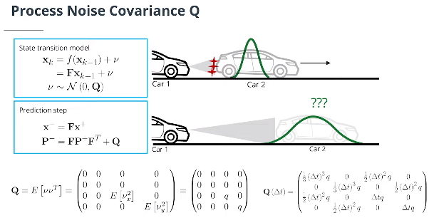
如果假设对于$x$和$y$方向加速度的噪声相等，即$\nu_x=\nu_{y}$，则连续过程噪声协方差可建模为：

\[\mathbf{Q}= E\left[\nu\nu^T\right] = \begin{pmatrix} 0 & 0 & 0 & 0 \\ 0 & 0 & 0 & 0 \\ 0 & 0 & E\left[\nu_{ x}^2\right] & 0 \\ 0 & 0 & 0 & E\left[\nu_{ y}^2\right] \end{pmatrix} = \begin{pmatrix} 0 & 0 & 0 & 0 \\ 0 & 0 & 0 & 0 \\ 0 & 0 & q & 0 \\ 0 & 0 & 0 & q \end{pmatrix}\]

将该连续模型离散化后，根据$Δt$得出$\mathbf Q$的公式如下：

\[\mathbf Q \left(\Delta t\right) = \int_0^{\Delta t}\mathbf{F}\left(t\right)\mathbf{Q}\mathbf{F}\left(t\right)^T dt = \int_0^{\Delta t} \begin{pmatrix} 1 & 0 & t & 0 \\ 0 & 1 & 0 & t \\ 0 & 0 & 1 & 0 \\ 0 & 0 & 0 & 1 \end{pmatrix} \begin{pmatrix} 0 & 0 & 0 & 0 \\ 0 & 0 & 0 & 0\\ 0 & 0 & q & 0 \\ 0 & 0 & 0 & q \end{pmatrix} \begin{pmatrix} 1 & 0 & 0 & 0 \\ 0 & 1 & 0 & 0 \\ t & 0 & 1 & 0 \\ 0 & t & 0 & 1 \end{pmatrix} dt\] \[= \int_0^{\Delta t}\begin{pmatrix} t^2 q & 0 & t q & 0 \\ 0 & t^2 q & 0 & t q\\ 0 & 0& q & 0 \\ 0 & 0 & 0 & q \end{pmatrix} dt =\begin{pmatrix} \frac 1{3} \left(\Delta t\right)^3 q & 0 & \frac 1{2} \left(\Delta t\right)^2 q& 0 \\ 0 & \frac 1{3} \left(\Delta t\right)^3 q& 0 & \frac 1{2} \left(\Delta t\right)^2 q\\ \frac 1{2} \left(\Delta t\right)^2 q& 0 & \Delta t q& 0 \\ 0 & \frac 1{2} \left(\Delta t\right)^2 q& 0 & \Delta t q \end{pmatrix}\]

此处$q$是一个设计参数，应根据预期的最大速度变化来选择。对于高动态运动模型，我们可以使用更高的过程噪音， $q=\left(8\,\frac{\text m}{s^2}\right)^2$ 对于高度不确定的运动对象来说比较合适，能用于紧急制动。而对于高速公路上的正常情况，例如$q=\left(3\,\frac{\text m}{s^2}\right)^2$ 可能是一个适当的选择。

5.2 更新步骤–激光雷达测量（2维KF）

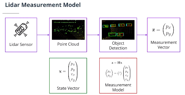
• 测量向量

$z$是测量向量。对于激光雷达传感器，$\mathbf z$向量包含$x$和$y$中的位置测量值：

\[\mathbf z = \begin{pmatrix} p_x\\p_y \end{pmatrix}\]

$H$ 是将对对象当前状态的信念投射到传感器测量空间的矩阵。对于激光雷达来说，这是一种奇特的说法，即我们丢弃状态变量中的速度信息，因为激光雷达传感器仅测量位置：状态向量$\mathbf x$包含关于$\begin{pmatrix}p_x，p_y，v_x，v_y\end{pmatrix}$的信息，而$\mathbf z$向量将只包含$\begin{pmatrix}p_x，p_y\end{pmatrix}$.乘以$\mathbf H\mathbf x$，我们可以将$\mathbf x$（我们的预测状态）与 $\mathbf z$（传感器测量值）进行比较。

• 从4D状态空间投影到2D测量空间的$\mathbf H$矩阵

\[\begin{pmatrix} p_x\\p_y \end{pmatrix} = \mathbf H \begin{pmatrix} p_x\\p_y\\v_x\\v_y \end{pmatrix}\] \[\mathbf H = \begin{pmatrix} 1 & 0 & 0 & 0 \\ 0 & 1 & 0 &0 \end{pmatrix}\] \[\begin{pmatrix} p_x\\p_y \end{pmatrix} = \begin{pmatrix} 1 & 0 & 0 & 0 \\ 0 & 1 & 0 &0 \end{pmatrix} \begin{pmatrix} p_x\\p_y\\v_x\\v_y \end{pmatrix}\]

• 测量噪声协方差矩阵R

测量噪声协方差矩阵R代表传感器测量中的不确定性。R矩阵的尺寸为正方形，其矩阵的每一侧的长度与测量参数的数量相同。对于激光雷达传感器，我们有一个二维测量向量。每个位置 $\left(p_x, p_y\right)$都受到随机噪声的影响。因此，我们的噪声向量$\omega$与$\mathbf z$的维数相同。它是一个均值为零，协方差矩阵是垂直向量ω与其转置的乘积形成的2 x 2矩阵的分布。

\[\mathbf R = E[\omega \omega^T] = \begin{pmatrix} \sigma^2_{x} & 0 \\ 0 & \sigma^2_{y} \end{pmatrix}\]

其中$\textbf R$是测量噪声协方差矩阵。换句话说，$\textbf R$矩阵表示我们从激光雷达传感器接收到的位置测量的不确定性。通常，测量噪声协方差矩阵的参数将由传感器制造商提供，或必须在路试中确定。 $\textbf R$中的非对角0表示我们假设噪声过程不相关，$x$位置的噪声不会影响$y$位置，反之亦然。

Python实现激光雷达卡尔曼滤波2D对象追踪

import numpy as np
import matplotlib
matplotlib.use('wxagg') # change backend so that figure maximizing works on Mac as well  
import matplotlib.pyplot as plt

class Filter:
    '''Kalman filter class'''
    def __init__(self):
        self.dim_state = 4 # process model dimension
        self.dt = 0.1 # time increment
        self.q=0.1 # process noise variable for Kalman filter Q

    def F(self):
        # system matrix
        dt = self.dt
        return np.matrix([[1, 0, dt, 0],
                        [0, 1, 0, dt],
                        [0, 0, 1, 0],
                        [0, 0, 0, 1]])

    def Q(self):
        # process noise covariance Q
        q = self.q
        dt = self.dt
        q1 = ((dt**3)/3) * q 
        q2 = ((dt**2)/2) * q 
        q3 = dt * q 
        return np.matrix([[q1, 0, q2, 0],
                        [0, q1, 0, q2],
                        [q2, 0, q3, 0],
                        [0, q2, 0,  q3]])

    def H(self):
        # measurement matrix H
        return np.matrix([[1, 0, 0, 0],
                       [0, 1, 0, 0]]) 

    def predict(self, x, P):
        # predict state and estimation error covariance to next timestep
        F = self.F()
        x = F*x # state prediction
        P = F*P*F.transpose() + self.Q() # covariance prediction
        return x, P

    def update(self, x, P, z, R):
        # update state and covariance with associated measurement
        H = self.H() # measurement matrix
        gamma = z - H*x # residual
        S = H*P*H.transpose() + R # covariance of residual
        K = P*H.transpose()*np.linalg.inv(S) # Kalman gain
        x = x + K*gamma # state update
        I = np.identity(self.dim_state)
        P = (I - K*H) * P # covariance update
        return x, P     


def run_filter():
    ''' loop over data and call predict and update'''
    np.random.seed(0) # make random values predictable

    # init filter
    KF = Filter()

    # init figure
    fig, ax = plt.subplots()

    # init track state and covariance
    x = np.matrix([[0],
                [0],
                [0],
                [0]])
    P = np.matrix([[0.1**2, 0, 0, 0],
                [0, 0.1**2, 0, 0],
                [0, 0, 2**2, 0],
                [0, 0, 0, 2**2]])

    # loop over measurements and call predict and update
    for i in range(1,101):        

        # prediction
        x, P = KF.predict(x, P) # predict to next timestep

        # ground truth generation
        gt = np.matrix([[i*KF.dt], 
                       [0.1*(i*KF.dt)**2]])

        # measurement generation
        sigma_z = 0.2 # measurement noise 
        z = np.matrix([[float(gt[0]) + np.random.normal(0, sigma_z)],
                       [float(gt[1]) + np.random.normal(0, sigma_z)]]) # generate noisy measurement
        R = np.matrix([[sigma_z**2, 0], # measurement noise covariance matrix
                            [0, sigma_z**2]])

        # update
        x, P = KF.update(x, P, z, R) # update with measurement

        # visualization    
        ax.scatter(float(x[0]), float(x[1]), color='green', s=40, marker='x', label='track')
        ax.scatter(float(z[0]), float(z[1]), color='blue', marker='.', label='measurement')
        ax.scatter(float(gt[0]), float(gt[1]), color='gray', s=40, marker='+', label='ground truth')
        ax.set_xlabel('x [m]')
        ax.set_ylabel('y [m]')
        ax.set_xlim(0,10)
        ax.set_ylim(0,10)

        # maximize window        
        mng = plt.get_current_fig_manager()
        mng.frame.Maximize(True) 

        # remove repeated labels
        handles, labels = ax.get_legend_handles_labels()
        handle_list, label_list = [], []
        for handle, label in zip(handles, labels):
            if label not in label_list:
                handle_list.append(handle)
                label_list.append(label)
        ax.legend(handle_list, label_list, loc='center left', shadow=True, fontsize='x-large', bbox_to_anchor=(0.8, 0.5))

        plt.pause(0.01)
    plt.show()


####################
# call main loop
run_filter()

5.3 更新步骤–相机测量数据更新（2维EKF）

• 针孔相机模型

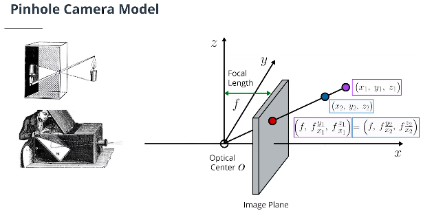
三维点到二维图像平面的投影公式：

\[\begin{pmatrix}x，&y，&z\end{pmatrix}\mapsto\Large\begin{pmatrix}\frac{f\cdot y}{x}，&\frac{f\cdot z}{x}\end{pmatrix}\]

这表明距离信息丢失，需要通过传感器融合来补偿损失。

• 相机测量模型

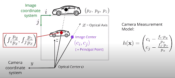
$(c_i,c_j)$ 是图像坐标中的图像中心或主要点，由内部摄像机校准导出。

$(f_i,f_j)$ 是从内部摄像机校准导出的图像坐标中的焦距。

将3D点（或6D状态向量，因为我们忽略了速度分量）投影到2D图像空间会得到以下非线性测量函数：

\[h(\mathbf{x}) = h\left(\begin{pmatrix} p_x\\ p_y\\ p_z\\ v_x\\ v_y\\ v_z \end{pmatrix}\right) = \Large \begin{pmatrix} c_i-\frac{f_i\cdot p_y}{p_x}\\ c_j-\frac{f_j\cdot p_z}{p_x} \end{pmatrix}\]

激光雷达中的$\textbf H$矩阵和相机中的$h（\mathbf x）$函数实际上完成了相同的任务：它们都用于计算更新步骤中的残差$\gamma=\mathbf z-\mathbf H\mathbf x$。

但对于相机，没有 $\textbf H$ 矩阵将状态向量$\textbf X$映射到图像坐标;相反需要手动计算从笛卡尔坐标转换为图像坐标的映射。

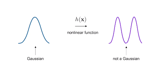
因此，对于相机来说$\gamma=\mathbf z-\mathbf H\mathbf x$变成$\gamma=\mathbf z-h（\mathbf x）$。$h$是一个非线性函数。

• 扩展卡尔曼滤波器（EKF）

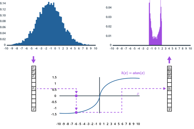
点$μ$处方程$h（x）$的泰勒级数展开式的一般形式如下：

\[h(x) = h(\mu) + h'(\mu) ( x - \mu)+ \frac{h''(\mu)}{2!} ( x - \mu)^2+...,\]

$n!$表示$n$的阶乘。如果$\mu$接近$x$，$（x-\mu）^2$以及更高阶项变得很小，所以我们可以忽略它们。因此，我们得到：

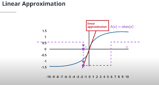
\[h(x) \approx h(\mu) + h'(\mu) ( x - \mu).\]

简单地用一个给定的方程替换$h（x）$，求导数，并插入值$\mu$，以找到该点$\mu$的泰勒展开式。

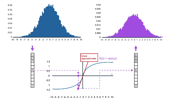
看看是否可以找到$\arctan（x）$的泰勒展开式！假设我们有一个平均值为$\mu = 0$的预测状态，将预测状态$x$投影到测量空间的函数为：$h(x) = \arctan(x)$ ，它的导数是：$h’(x) = \frac 1{1+ x^2}$ ，用一阶泰勒展开来求出在平均位置$\mu=0$处使函数$h（x）$线性化的线性近似函数是$h(x) \approx x$ 。当$\mu=0$时，$h(x) \approx \arctan(0) + \frac{1}{1+0}(x-0) = x$， 因此，函数 $h(x) = \arctan(x)$ 将被线: $h(x) \approx x$近似逼近。

• 多元泰勒级数

了解了如何用一维方程进行泰勒级数展开，接下来看多维方程的泰勒级数展开。相机测量函数$h$函数由两个方程组成，这两个方程显示了预测状态$\mathbf x$如何映射到图像空间：

\[h(\mathbf{x}) = h\left(\begin{pmatrix} p_x\\ p_y\\ p_z\\ v_x\\ v_y\\ v_z \end{pmatrix}\right) = \Large \begin{pmatrix} c_i-\frac{f_i\cdot p_y}{p_x}\\ c_j-\frac{f_j\cdot p_z}{p_x} \end{pmatrix}\]

这些是多维方程组，因此需要使用多维泰勒级数展开来对h函数进行线性近似。以下是多维泰勒级数展开的一般公式：

\[h(x) \approx h(\mu) + \mathbf H_J(\mu) ( x - \mu)\]

这里我们简单地用雅可比矩阵$\mathbf H_J(\mu)$替换了一阶导数$h’（\mu）$. 雅可比矩阵包含多维函数$h$的偏导数。

• 雅可比矩阵 $\mathbf H_J$推导

这是用于相机测量的雅可比矩阵 $\mathbf H_J$ 的完整推导。重要的是理解线性化的总体思想，并能够实现得到的雅可比矩阵。将6D状态向量投影到2D图像空间要能够提供以下非线性相机测量功能：

\[h(\mathbf{x}) = h\left(\begin{pmatrix} p_x\\ p_y\\ p_z\\ v_x\\ v_y\\ v_z \end{pmatrix}\right) = \large \begin{pmatrix} c_i-\frac{f_i\cdot p_y}{p_x}\\ c_j-\frac{f_j\cdot p_z}{p_x} \end{pmatrix} = \begin{pmatrix} h_1(\mathbf x)\\ h_2(\mathbf x) \end{pmatrix}\]

因此，我们要寻找一个2x6维度的雅可比矩阵$H_J$：

\[\mathbf H_J = \Large \begin{pmatrix} \frac{\partial h_1(\mathbf x)}{\partial p_x}& \frac{\partial h_1(\mathbf x)}{\partial p_y}& \frac{\partial h_1(\mathbf x)}{\partial p_z}& \frac{\partial h_1(\mathbf x)}{\partial v_x}& \frac{\partial h_1(\mathbf x)}{\partial v_y}& \frac{\partial h_1(\mathbf x)}{\partial v_z}\\ \frac{\partial h_2(\mathbf x)}{\partial p_x}& \frac{\partial h_2(\mathbf x)}{\partial p_y}& \frac{\partial h_2(\mathbf x)}{\partial p_z}& \frac{\partial h_2(\mathbf x)}{\partial v_x}& \frac{\partial h_2(\mathbf x)}{\partial v_y}& \frac{\partial h_2(\mathbf x)}{\partial v_z} \end{pmatrix}\]

可以计算$\mathbf H_J$的所有条目详情如下:

\[\frac{\partial h_1(\mathbf x)}{\partial p_x} = \partial p_x \left(c_i-\frac{f_i\cdot p_y}{p_x}\right) = \frac{f_i\cdot p_y}{p_x^2}\] \[\frac{\partial h_1(\mathbf x)}{\partial p_y} = \partial p_y \left(c_i-\frac{f_i\cdot p_y}{p_x}\right) = -\frac{f_i}{p_x}\] \[\frac{\partial h_1(\mathbf x)}{\partial p_z} = \partial p_z \left(c_i-\frac{f_i\cdot p_y}{p_x}\right) = 0\] \[\frac{\partial h_2(\mathbf x)}{\partial p_x} = \partial p_x \left(c_j-\frac{f_j\cdot p_z}{p_x}\right) = \frac{f_j\cdot p_z}{p_x^2}\] \[\frac{\partial h_2(\mathbf x)}{\partial p_y} = \partial p_y \left(c_j-\frac{f_j\cdot p_z}{p_x}\right) = 0\] \[\frac{\partial h_2(\mathbf x)}{\partial p_z} = \partial p_z\left(c_j-\frac{f_j\cdot p_z}{p_x}\right) = -\frac{f_j}{p_x}\]

此外，速度分量之后的所有导数都为零，因为测量函数中未使用速度。总结一下，雅可比 $\mathbf H_J$是：

\[\mathbf H_J = \large \begin{pmatrix} \frac{f_i\cdot p_y}{p_x^2} & -\frac{f_i}{p_x} & 0& 0& 0& 0\\ \frac{f_j\cdot p_z}{p_x^2} & 0& -\frac{f_j}{p_x} & 0& 0& 0 \end{pmatrix}\]

Python 实现相机测量模型的雅克比矩阵

import numpy as np
import matplotlib
matplotlib.use('wxagg') # change backend so that figure maximizing works on Mac as well  
import matplotlib.pyplot as plt

class Camera:
    '''Camera sensor class including measurement matrix'''
    def __init__(self):
        self.f_i = 2095.5 # focal length i-coordinate
        self.f_j = 2095.5 # focal length j-coordinate
        self.c_i = 944.9 # principal point i-coordinate
        self.c_j = 640.2 # principal point j-coordinate 

    def get_hx(self, x):    
        # calculate nonlinear measurement expectation value h(x)   
        hx = np.zeros((2,1))
        # check and print error message if dividing by zero
        if x[0]==0:
            raise NameError('Jacobian not defined for x[0]=0!')
        else:
            hx[0,0] = self.c_i - self.f_i*x[1]/x[0] # project to image coordinates
            hx[1,0] = self.c_j - self.f_j*x[2]/x[0]
            return hx    

    def get_H(self, x):
        # calculate Jacobian H at current x from h(x)
        H = np.matrix(np.zeros((2, 6)))
        # check and print error message if dividing by zero
        if x[0]==0:
            raise NameError('Jacobian not defined for x[0]=0!')
        else:
            H[0,0] = self.f_i * x[1] / (x[0]**2)
            H[1,0] = self.f_j * x[2] / (x[0]**2)
            H[0,1] = -self.f_i / x[0]
            H[1,2] = -self.f_j / x[0]
            return H

def calc_Jacobian(x):
    # calculate Jacobian for x
    cam = Camera()
    H = cam.get_H(x)

    # init visualization
    fig, (ax1, ax2) = plt.subplots(1,2)
    plot_x = []
    plot_y1 = []
    plot_y2 = []
    lin_y1 = []
    lin_y2 = []

    # calculate Taylor series expansion point
    hx_orig = cam.get_hx(x)
    ax1.plot(x[0], hx_orig[0], marker='x', color='green', label='expansion point x')
    ax2.plot(x[0], hx_orig[1], marker='x', color='green', label='expansion point x')

    # calculate linear approximation at this point 
    s1 = float(H[0,0]) # slope of tangent given by Jacobian H
    s2 = float(H[1,0])
    i1 = float(hx_orig[0] - s1*x[0]) # intercept i = y - s*x
    i2 = float(hx_orig[1] - s2*x[0])

    # calculate nonlinear measurement function h
    for px in range(1,50):
        x[0] = px
        hx = cam.get_hx(x)
        plot_x.append(px)
        plot_y1.append(hx[0])
        plot_y2.append(hx[1])
        lin_y1.append(s1*px + i1)
        lin_y2.append(s2*px + i2)

    # plot results
    ax1.plot(plot_x, plot_y1, color='blue', label='measurement function h')
    ax1.plot(plot_x, lin_y1, color='red', label='linear approximation H')
    ax2.plot(plot_x, plot_y2, color='blue', label='measurement function h')
    ax2.plot(plot_x, lin_y2, color='red', label='linear approximation H')

    # maximize window     
    mng = plt.get_current_fig_manager()
    mng.frame.Maximize(True)

    # legend
    ax1.legend(loc='center left', shadow=True, fontsize='large', bbox_to_anchor=(0.5, 0.1))
    ax1.set_xlabel('x [m]')
    ax1.set_ylabel('h(x) first component [px]')
    ax2.legend(loc='center left', shadow=True, fontsize='large', bbox_to_anchor=(0.5, 0.1))
    ax2.set_xlabel('x [m]')
    ax2.set_ylabel('h(x) second component [px]')

    plt.show()

#################
# define expansion point for Taylor series
x = np.matrix([[10],
            [1],
            [-1],
            [0],
            [0],
            [0]])

calc_Jacobian(x)

• 相机数据更新扩展卡尔曼滤波方程

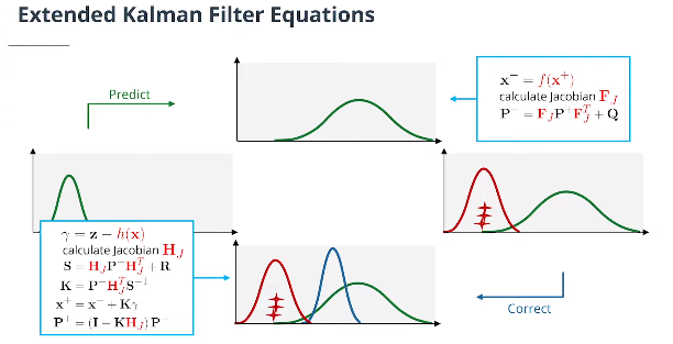
虽然数学证明有点复杂，但事实证明，卡尔曼滤波方程和扩展卡尔曼滤波方程非常相似。主要区别在于：

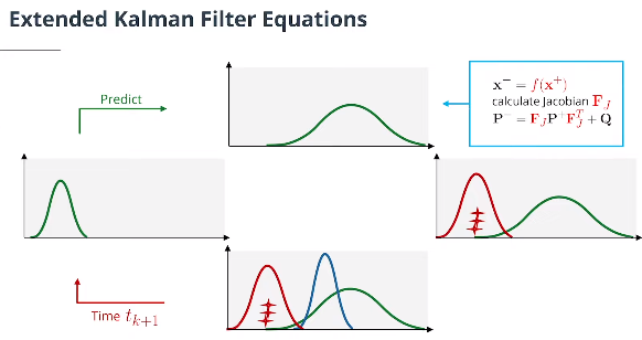
计算$\mathbf P^-$时，使用$\mathbf F_J$替换$\textbf F$矩阵

计算 $\mathbf S$, $\mathbf K$, $\mathbf P^+$时，使用$\mathbf H_J$替换$\textbf H$矩阵

计算$\mathbf x^-$，使用预测更新函数$f$替换$\textbf F$矩阵。

计算$\gamma$，使用测量函数$h$替换$\textbf H$矩阵。

但是，对于最终的项目，我们不需要使用$f$函数或$\mathbf F_J$，因为我们在预测步骤中使用了线性模型。因此，对于预测步骤，我们仍然可以使用常规卡尔曼滤波方程和$\textbf F$矩阵，而不是扩展卡尔曼滤波方程。

激光雷达的测量更新也将使用常规卡尔曼滤波方程，因为激光雷达使用线性方程。只有相机传感器的测量更新才会使用扩展卡尔曼滤波方程。

需要重申的一个重要点是卡尔曼滤波器的方程$\gamma=\mathbf z-\mathbf H\mathbf x$不会变成扩展卡尔曼滤波器$\gamma=\mathbf z-\mathbf H_J\mathbf x$。相反，对于扩展卡尔曼滤波器，我们将直接使用$h$函数从笛卡尔坐标直接映射到图像坐标的预测位置$\mathbf x^-$。

5.4 坐标转换与EKF传感器融合总结

• 坐标转换

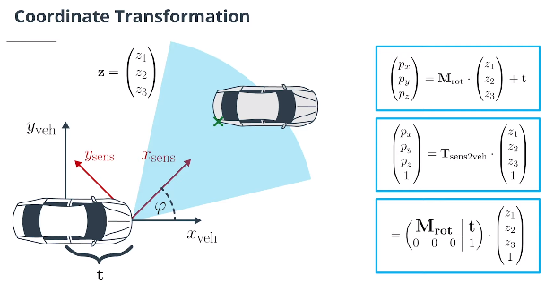
3x3 $\textbf{rotation matrix}$旋转矩阵 $\mathbf M_{\text{rot}}$ 和 3D 平移转换向量 $\textbf{translation vector}$ $\mathbf t$ 将传感器坐标转换为车辆坐标：

\[\begin{pmatrix} p_x\\ p_y\\p_z \end{pmatrix} = \mathbf M_{\text{rot}} \cdot \begin{pmatrix} z_1\\ z_2\\z_3 \end{pmatrix} +\mathbf t\]

注意：应用旋转和平移的顺序在这里很重要，这种转换很容易出错。因此，最好使用以下转换：

$\textbf{Transformation Matrix}$变换矩阵使用$\textbf{homogeneous coordinates}$齐次坐标将传感器坐标转换为车辆坐标：

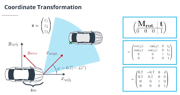
\[\begin{pmatrix} p_x\\ p_y\\p_z\\1 \end{pmatrix} = \mathbf T_{\text{sens2veh}} \cdot \begin{pmatrix} z_1\\ z_2\\z_3\\1 \end{pmatrix} = \left(\begin{array}{c|c } {\large \mathbf M_{\text{rot}}} & {\large t} \\ \overline{\begin{matrix} 0 &0&0 \end{matrix}} & \overline {\begin{matrix} 1 \end{matrix}} \end{array}\right) \cdot \begin{pmatrix} z_1\\ z_2\\z_3\\1 \end{pmatrix} = \left(\begin{array}{c|c} \begin{matrix} r_{11} & r_{12}& r_{13} \\ r_{21} & r_{22}& r_{23}\\ r_{31} & r_{32}& r_{33} \end{matrix} & \begin{matrix} t_1 \\ t_2\\ t_3 \end{matrix}\\ \overline{ \begin{matrix} 0 &0&0 \end{matrix}} & \overline{\begin{matrix} 1 \end{matrix}} \end{array}\right) \cdot \begin{pmatrix} z_1\\ z_2\\z_3\\1 \end{pmatrix}\]

示例：在传感器位于后轴（=车辆坐标系原点）前方4m且旋转φ=0.7（$=45^{\circ}$）的左前方车辆，我们有以下转换矩阵：

\[\mathbf T_{\text{sens2veh}} = \left(\begin{array}{c|c} {\large \mathbf M_{\text{rot}}} & {\large \text t} \\ \overline{\begin{matrix} 0 &0&0 \end{matrix}} & \overline {\begin{matrix} 1 \end{matrix}} \end{array}\right) = \begin{pmatrix} \cos(\phi)& -\sin(\phi)& 0 &t_1 \\ \sin(\phi) & \cos(\phi)& 0& t_2\\ 0 & 0&1 & t_3\\ 0&0 & 0&1 \end{pmatrix} = \begin{pmatrix} 0.7& -0.7& 0 &4 \\ 0.7 & 0.7& 0& 0\\ 0 & 0&1 & 0\\ 0&0 & 0&1 \end{pmatrix}\]

从车辆到传感器坐标的变换矩阵 $\mathbf T_{\text{veh2sens}}$是$\mathbf T_{\text{sens2veh}}$的逆矩阵。

• EKF传感器融合总结

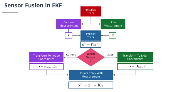
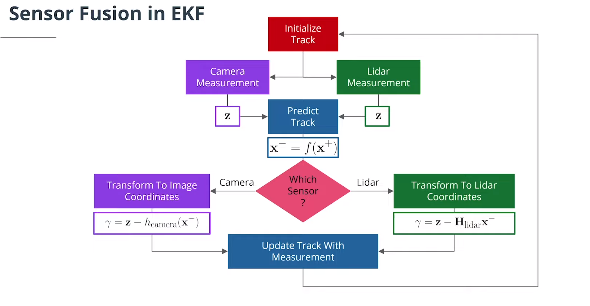
当新测量到达时，我们执行以下步骤：

计算时间步长$\Delta t$和新的状态转移矩阵$\mathbf F$和过程噪声协方差矩阵$\mathbf Q$。

预测下一个时间戳的状态和协方差。

将状态从车辆坐标转换为传感器坐标。

对于相机测量，使用非线性测量模型并计算新的雅可比矩阵，否则使用线性测量模型更新状态和协方差。